tidydiversity

Taxonomic, phylogenetic and functional diversity on one scale, in one tidy workflow.

Reviewers increasingly expect taxonomic (TD), phylogenetic (PD) and functional (FD) diversity to be reported together and to be comparable. tidydiversity expresses all three as Hill numbers of the same order q, in units of effective numbers of species, and standardises them by sample size or sample coverage. Data go in as a long data frame and results come back as tibbles.

In memory of Filip Damen (about 1966-2026). tidydiversity is dedicated to the Wanang leader who refused the loggers, kept his forest for science, and built a research station, a school and a health post with his community. The wanang_butterflies data come from the forest he protected. Read his story.

Taxonomic (TD)

Species counts only. Observed and asymptotic Hill numbers, sample coverage, rarefaction and extrapolation, matching iNEXT.

Phylogenetic (PD)

Add a phylogeny with type = "PD", tree = tree. Effective number of lineages at a reference time, matching iNEXT.3D.

Functional (FD)

Add a trait distance matrix with type = "FD", distance = d. Effective number of functionally distinct species at a threshold tau, or the area under the tau profile, matching iNEXT.3D.

Why tidydiversity?

Community ecology in R is spread over many packages: iNEXT and iNEXT.3D for Hill numbers, vegan for ordination and permutation tests, betapart for beta diversity, FD, TPD, ade4 and phytools for traits and phylogenies. Each has its own input format (wide matrices, lists, row names) and its own output (lists, S4 objects, printed tables). Most of an analysis ends up as glue code: reshaping data frames by hand, matching species names across matrices, pulling numbers out of nested lists, and re-drawing every plot. tidydiversity replaces that glue with one consistent, tested interface.

One workflow instead of hand-rolled glue

You usually hand-roll	With tidydiversity
Pivot long field data to a site x species matrix, align row names with the site table	Long data in, one row per site and species: div_hill(data, site, species, abundance)
Match species names between the community matrix, the trait table and the tree	Matched and checked for you, with a clear error naming the missing species
Loop over seasons or treatments and bind the results	.by = season, or group_by()
Dig estimates out of iNEXT, vegan or FD list objects	Every result is a tibble; tidy() and glance() for models
Rebuild CANOCO-style biplots, rarefaction curves and multi-panel figures	autoplot(), plot_panel(), plot_save() at journal sizes
Write permutation tests for CWM, null models, forward selection	trait_cwm_test() (max test), trait_ses(), ord_select()
Feed diversity into tidymodels with leakage-free resampling	model_group_folds(), model_case_weights(), step_hill()

Gaps it fills

• TD, PD and FD on one scale. Taxonomic, phylogenetic and functional Hill numbers of the same order q, in effective numbers of species, standardised by sample size or coverage (Chao et al. 2014, 2019).
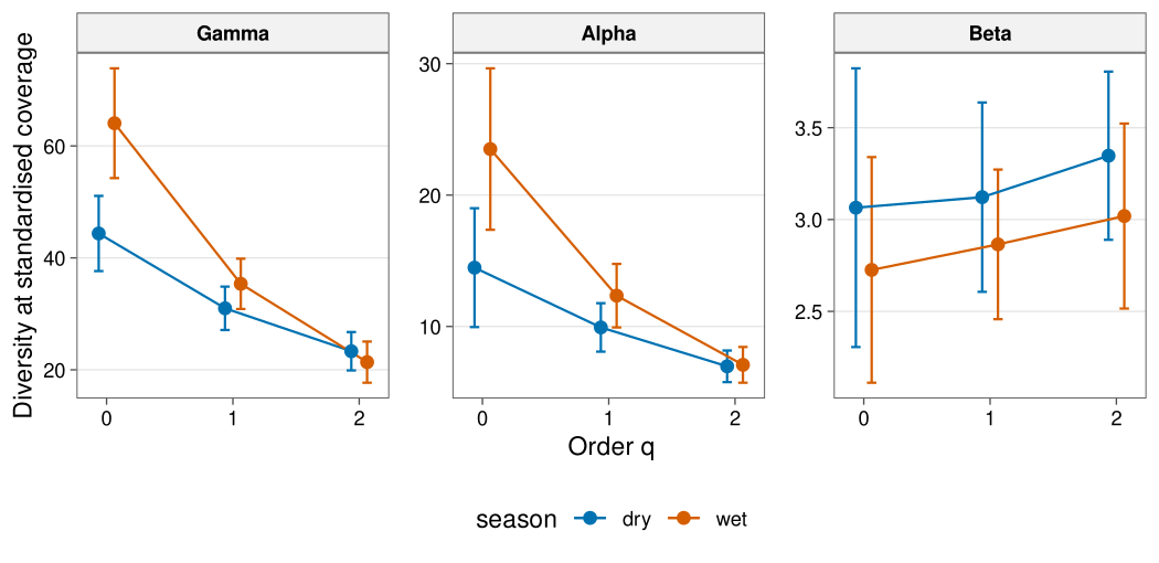
• Beta diversity at equal coverage. Gamma, alpha and beta Hill numbers and four normalised dissimilarities for TD, PD and FD, standardised to a common sample coverage with bootstrap intervals (beta_hill(), Chao et al. 2023), so regions sampled with unequal effort can be compared.
• Current, accepted methods. The max test for community-weighted means (Zeleny 2018), forward selection with double stopping (Blanchet et al. 2008), adjusted R² variation partitioning, trait probability densities (Carmona et al. 2019), gawdis trait distances (de Bello et al. 2021), Rao partitioning in equivalent numbers, and the full trait workflow of the Handbook of Trait-Based Ecology.
• Statistics that respect the design. Restricted permutations within blocks, a Welch-type PERMANOVA that stays valid when groups differ in spread (beta_welch(), Hamidi et al. 2019), site-blocked cross-validation, and precision weights from estimation error.
• Publication output. CANOCO-style biplots and triplots with ellipses, hulls and spiders; consistent colour-blind-safe themes on white backgrounds; multi-panel figures with panel tags.
• ForestGEO censuses. Tidy stem tables, basal area, size classes, census demography (mortality, recruitment, growth) and stems as a community table, ready for every div_ and beta_ verb.
• Maps live in tidymapr. Study-site maps, basemaps, rasters, bioclim layers, spatial statistics and species distribution models are in the companion package tidymapr, which takes the same tidy tables and returns the same tibbles and ggplots.

Fast where it matters

Hot loops are rewritten as compiled C++ (Rcpp) kernels or as vectorised matrix algebra. Every rewrite is tested against the reference package and gives identical results. Timings on one CPU core, with the Brazil rainforest data of iNEXT.3D (3868 individuals, 425 species, 40 sample sizes) and the DaPhnE tree (1641 species):

Task	Before	tidydiversity	How
PD rarefaction and extrapolation	3.9 s	0.4 s	C++ hypergeometric kernel
FD rarefaction and extrapolation	3.6 s (iNEXT.3D)	0.2 s	C++ kernel
Blomberg’s K with 999 randomisations	4.4 s per K (phytools)	1.5 s in total	contrasts with precomputed tree terms
Community TPDs and TPD indices	2.5 s (TPD)	< 0.1 s	matrix algebra

Optional packages (vegan, FD, ade4, TPD, phytools, tidymodels) load only when a function needs them, so library(tidydiversity) stays light.

Made for the tidyverse

• Tidy in, tidy out. One row per site and species goes in, a tibble comes out, ready for dplyr, tidyr and ggplot2.
• Data-masking. Name your columns with site, species and abundance, as you would in dplyr.
• Grouping. Every verb takes .by and respects group_by().
• broom and tidymodels. tidy() and glance() methods, a recipes step, and rsample folds.
• ggplot2. autoplot() returns ordinary ggplot objects you can extend with +; patchwork composes them.
• Predictable names. Functions are grouped by prefix: div_ (alpha diversity), beta_, ord_, trait_, phylo_, model_, stems_ and plot_.
• Checked. Results match iNEXT, iNEXT.3D, betapart, vegan, FD, ade4, iNEXT.beta3D, indicspecies, TPD and phytools in more than 400 tests.

What one package covers

Topic	tidydiversity	Usually needs
Hill numbers, coverage, rarefaction/extrapolation (TD, PD, FD)	div_*()	iNEXT, iNEXT.3D, hillR
Beta diversity partitioning, distance decay and decay models	beta_pair(), beta_multi(), beta_decay(), beta_decay_model()	betapart
Pairwise Hill-number dissimilarity (Sorensen, Jaccard, Horn, Morisita-Horn)	beta_hill_pair()	vegan
Coverage-standardised beta diversity (TD, PD, FD)	beta_hill()	iNEXT.beta3D
Ordination (PCA to db-RDA) with biplots	ord_fit(), autoplot()	vegan, ggvegan, ggord
PERMANOVA (classic and Welch-type), dispersion, variation partitioning, forward selection	beta_permanova(), beta_welch(), beta_dispersion(), ord_varpart(), ord_select()	vegan, adespatial
Indicator species, corrected for multiple testing	beta_indicator()	indicspecies
Traits: CWM, FD indices, null models, ITV, fourth corner	trait_*()	FD, gawdis, picante, cati, ade4, weimea
Trait probability densities	trait_tpd()	TPD
Phylogenetic signal and distances	phylo_*()	phytools, picante, ape
Modelling with tidymodels	model_*(), step_hill()	hand-written glue
ForestGEO census tables and demography	stems_*()	fgeo, CTFS R package
Partial-effect and surface plots; overdispersed counts	plot_partial(), plot_surface(), model_count()	visreg, plotmo, aods3
Publication figures and tables	autoplot(), plot_*(), div_table()	ggplot2, patchwork, gt

Installation

Install the development version from GitHub:

# install.packages("pak")
pak::pak("jmozez/tidydiversity")

The source code lives on GitHub, https://github.com/jmozez/tidydiversity, with a mirror on GitLab, https://gitlab.com/jimmy.moses/tidydiversity.

Maps with tidymapr

tidydiversity does no geospatial work. Its companion package tidymapr draws study-site and diversity maps, reads and writes vector and raster files, downloads climate, elevation and boundary layers, computes spatial statistics and fits species distribution models. It takes the tidy tables tidydiversity uses and returns tibbles and ggplots, so the two packages share one workflow, the way dplyr and ggplot2 do:

pak::pak("jmozez/tidymapr")
library(tidydiversity)
library(tidymapr)

div_estimate(png_ants, q = 0, .by = season) |>
  dplyr::filter(season == "dry") |>
  dplyr::left_join(geo_example_sites(), by = "site") |>
  plot_geo(estimate, lon, lat, label = site)

Example

png_ants records ground-foraging ants at nutrient baits along the Mt Wilhelm elevational gradient in Papua New Guinea, in the dry and the wet season (Moses et al. 2023). Each row is one species at one bait, so diversity is estimated from the number of baits at which each species was found.

library(tidydiversity)
library(dplyr)

div_hill(png_ants, q = c(0, 1, 2), .by = season)
#> # A tibble: 30 x 5
#>    season site       q     n diversity
#>    <chr>  <chr>  <dbl> <dbl>     <dbl>
#>  1 dry    MW0200     0    47     16   
#>  2 dry    MW0200     1    47     12.3 
#>  3 dry    MW0200     2    47      9.91
#>  4 wet    MW0200     0    76     21   
#>  5 wet    MW0200     1    76     10.9 
#>  6 wet    MW0200     2    76      6.99
#>  7 dry    MW0700     0    23     15   
#>  8 dry    MW0700     1    23     11.8 
#>  9 dry    MW0700     2    23      8.67
#> 10 wet    MW0700     0    58     28   
#> # i 20 more rows

Compare sites at equal sample completeness. By default each season is standardised to the lowest coverage that all its sites reach at twice their sample size, so no site is extrapolated too far:

set.seed(1)
div_standardise(png_ants, .by = season, nboot = 50) |>
  filter(q == 0)
#> # A tibble: 10 x 10
#>    season site       q      m method        coverage diversity    se lower upper
#>    <chr>  <chr>  <dbl>  <dbl> <chr>            <dbl>     <dbl> <dbl> <dbl> <dbl>
#>  1 dry    MW0200     0  11.6  rarefaction      0.565      7.96 0.458  7.07  8.86
#>  2 wet    MW0200     0  45.1  rarefaction      0.796     15.7  1.42  12.9  18.4 
#>  3 dry    MW0700     0  46.0  extrapolation    0.565     26.0  5.31  15.6  36.4 
#>  4 wet    MW0700     0 116    extrapolation    0.796     42.2  6.36  29.8  54.7 
#>  5 dry    MW1200     0  11.0  rarefaction      0.565      7.17 0.669  5.86  8.48
#>  6 wet    MW1200     0  40.6  rarefaction      0.796     17.1  1.82  13.5  20.6 
#>  7 dry    MW1700     0   3.07 rarefaction      0.565      2.32 0.226  1.88  2.77
#>  8 wet    MW1700     0  25.4  rarefaction      0.796      8.36 1.58   5.26 11.5 
#>  9 dry    MW2200     0   4.76 rarefaction      0.565      3.48 0.363  2.77  4.20
#> 10 wet    MW2200     0   8.97 rarefaction      0.796      4.01 0.585  2.86  5.15

Example data from Papua New Guinea

Every example uses published field data, rebuilt from the original deposits by scripts in data-raw/.

Dataset	What it holds	Source
png_ants	Ants at nutrient baits, Mt Wilhelm, 200-3700 m, dry and wet season	Moses et al. (2023) Global Ecology and Biogeography, doi:10.1111/geb.13757
png_tree_ants	Every ant nest in 1254 trees at 200, 900 and 1800 m	Plowman et al. (2020) Ecography, doi:10.1111/ecog.04730
png_frogs	3390 frogs of 55 species at eight elevations, Mt Wilhelm	Dahl et al. (2024) Biotropica, doi:10.1111/btp.13283
wanang_butterflies	Butterflies on 36 days over three years, Wanang forest plot	Luk et al. (2019) Biotropica, doi:10.1111/btp.12671
wanang_caterpillars	9363 reared caterpillars of 849 morphospecies, primary and secondary forest at Wanang	Butterill and Redmond (2023) GBIF, doi:10.15468/7e96ht (CC BY 4.0)

TD, PD and FD on one scale

The same verbs give all three dimensions. Here are rarefaction and extrapolation curves for two Brazilian rainforest tree assemblages, using the abundance data, phylogeny and functional distances shipped with iNEXT.3D.

library(ggplot2)
data(list = c(
  "Brazil_rainforest_abun_data", "Brazil_rainforest_phylo_tree",
  "Brazil_rainforest_distance_matrix"
), package = "iNEXT.3D")
wide <- Brazil_rainforest_abun_data
brazil <- tibble(
  site = rep(colnames(wide), each = nrow(wide)),
  species = rep(rownames(wide), ncol(wide)),
  n = unlist(wide, use.names = FALSE)
) |>
  filter(n > 0)

curves <- bind_rows(
  div_rarefy(brazil, abundance = n, type = "TD") |> mutate(type = "TD"),
  div_rarefy(brazil,
    abundance = n, type = "PD",
    tree = Brazil_rainforest_phylo_tree
  ),
  div_rarefy(brazil,
    abundance = n, type = "FD",
    distance = as.matrix(Brazil_rainforest_distance_matrix)
  )
)

curves$type <- factor(curves$type, levels = c("TD", "PD", "FD"))

ggplot(curves, aes(m, diversity, colour = site)) +
  geom_line(aes(linetype = method == "extrapolation")) +
  geom_point(data = filter(curves, method == "observed"), size = 2) +
  facet_wrap(vars(q, type),
    ncol = 3, scales = "free_y",
    labeller = labeller(q = function(x) paste("q =", x), .multi_line = FALSE)
  ) +
  scale_linetype_manual(values = c("solid", "dashed"), guide = "none") +
  labs(
    x = "Number of individuals",
    y = "Effective number of species", colour = NULL
  ) +
  theme_tidydiversity()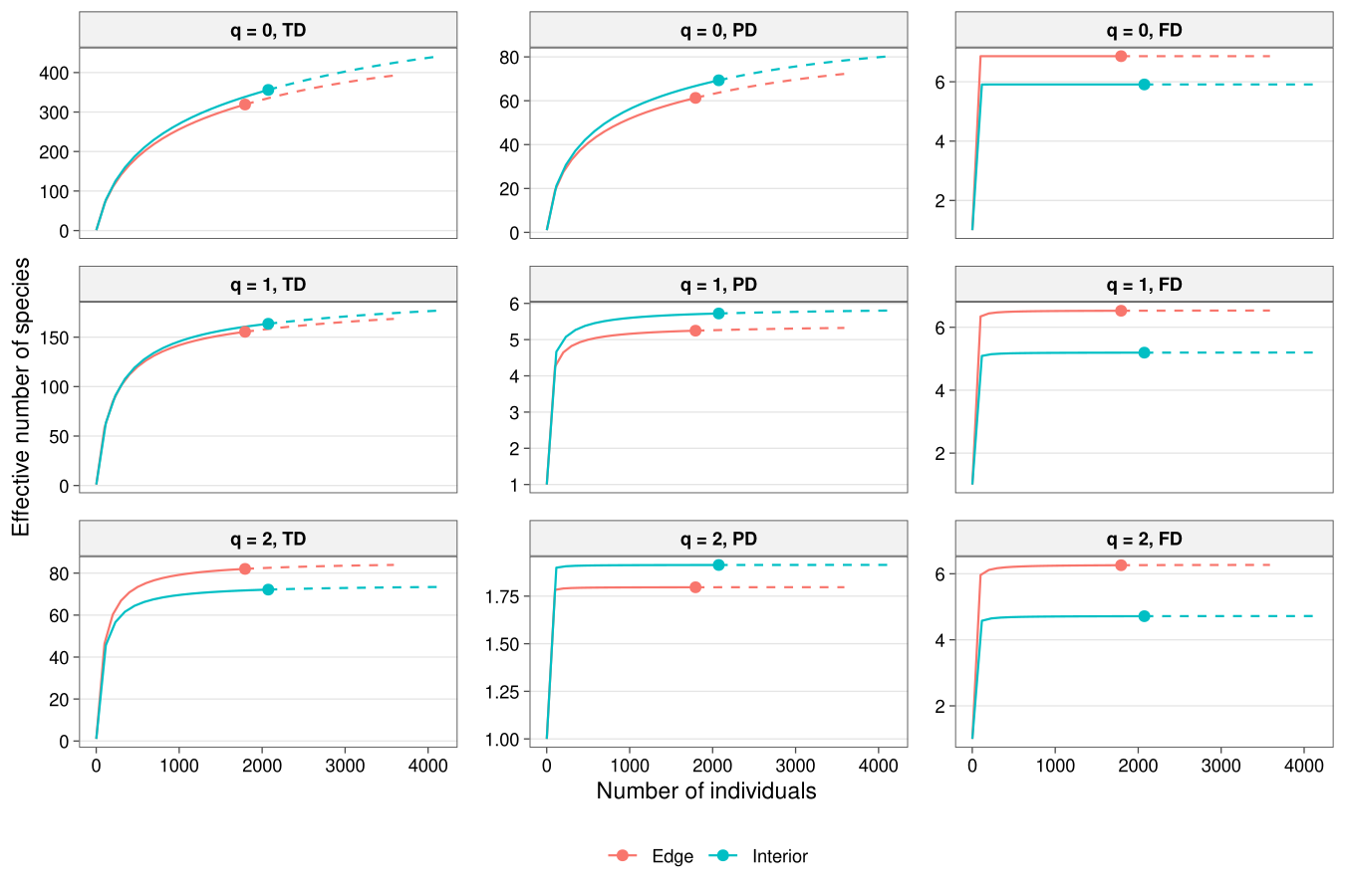

Why one scale?

Hill numbers of order q share one unit, the effective number of equally abundant (and, for PD and FD, equally distinct) species, so TD, PD and FD of the same order can be compared directly, and their ratios read as measures of phylogenetic or functional redundancy (Chao, Chiu and Jost 2014, doi:10.1146/annurev-ecolsys-120213-091540; Chao et al. 2019, doi:10.1002/ecm.1343). Standardising every dimension by the same sample size or coverage removes the effect of unequal sampling effort before you compare sites.

Functions

Family	Functions
Community data	as_community(), community_wide(), community_long(), add_site_data()
Alpha diversity (div_)	div_hill(), div_estimate(), div_coverage(), div_rarefy(), div_standardise(), div_completeness(), div_evenness(), div_boot()
Beta diversity (beta_)	beta_pair(), beta_multi(), beta_hill(), beta_hill_pair(), beta_decay(), beta_decay_model(), beta_dist(), beta_permanova(), beta_welch(), beta_dispersion(), beta_indicator()
Ordination (ord_)	ord_fit(), ord_test(), ord_select(), ord_varpart()
Traits (trait_)	trait_dist(), trait_cwm(), trait_cwm_test(), trait_fd_indices(), trait_rao(), trait_ses(), trait_itv(), trait_fourth_corner(), trait_tpd(), trait_tpd_dissim()
Phylogeny (phylo_)	phylo_signal(), phylo_dist(), phylo_combine_dist()
Modelling (model_)	model_group_folds(), model_case_weights(), step_hill(), tidy(), glance()
ForestGEO (stems_)	stems_as_trees(), stems_abundance(), stems_basal_area(), stems_size_class(), stems_demography(), stems_as_community()
Count models and partial plots	model_count(), plot_partial(), plot_surface()
Plots and tables (plot_)	autoplot(), plot_panel(), plot_save(), plot_palette(), plot_partial(), plot_surface(), plot_phylo(), plot_trait_space(), plot_venn(), theme_tidydiversity(), div_table()
Example data	png_ants, png_tree_ants, png_frogs, wanang_butterflies, wanang_caterpillars, data_aravo()

Gallery

Every plot that autoplot() draws, using png_ants.

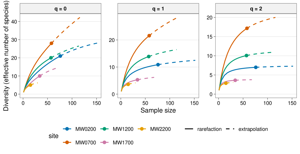
Rarefaction and extrapolation by sample size

Solid lines are rarefied, dashed lines extrapolated to twice the sample size; points are the observed samples (wet season).

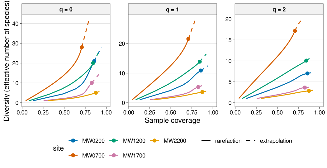
Rarefaction and extrapolation by sample coverage

The same curves plotted against estimated sample coverage, the basis for coverage-standardised comparison.

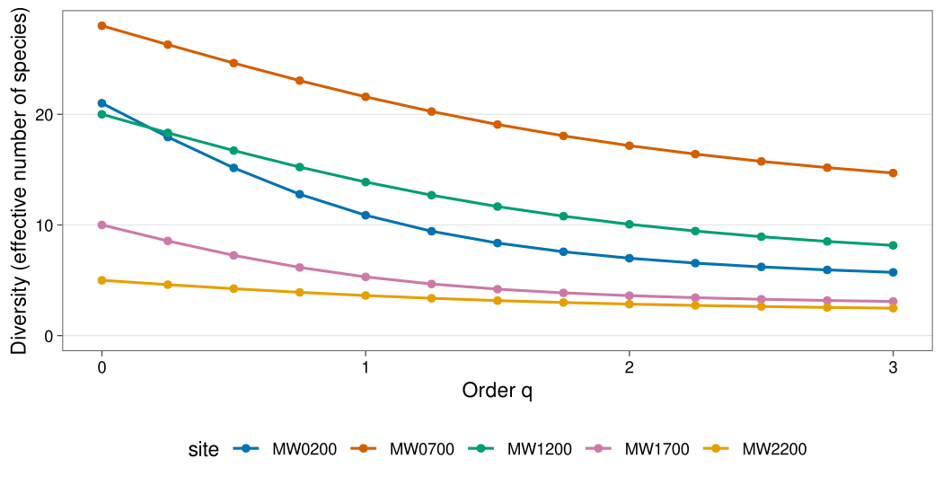
Hill diversity profile

Observed Hill numbers across orders q from 0 (richness) to 3 (dominant species), one line per site.

Alpha diversity along elevation

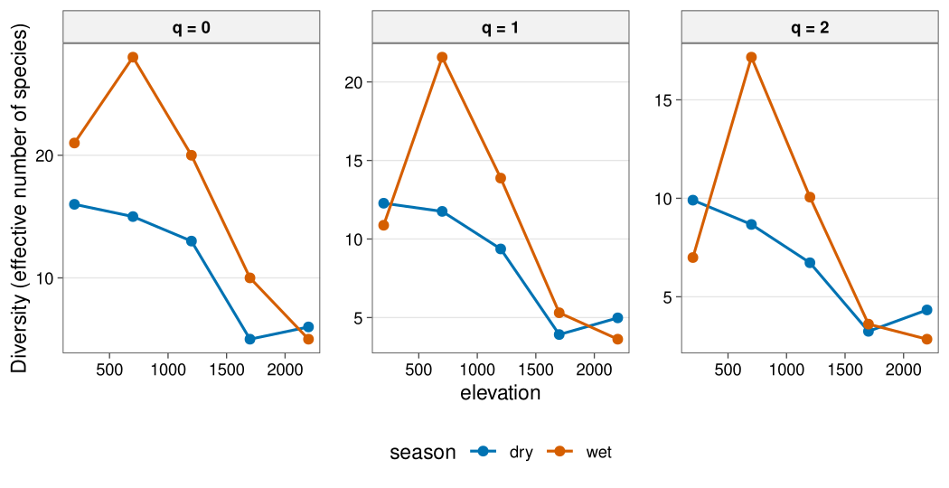
Observed q = 0, 1 and 2 diversity at each elevation, one line per season.

Observed and asymptotic diversity

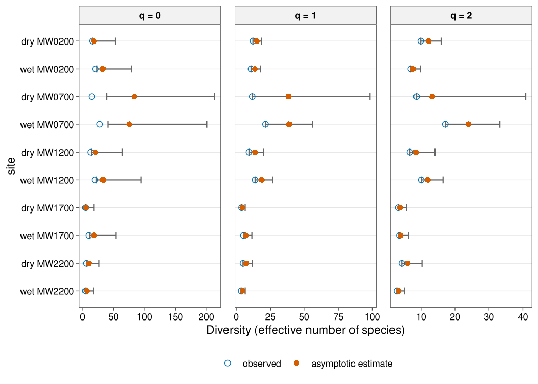
Open circles are observed values, filled circles the asymptotic estimates, with 95% bootstrap intervals.

Sample coverage

Estimated sample coverage of each site against its number of bait occurrences.

Pairwise beta diversity heatmap

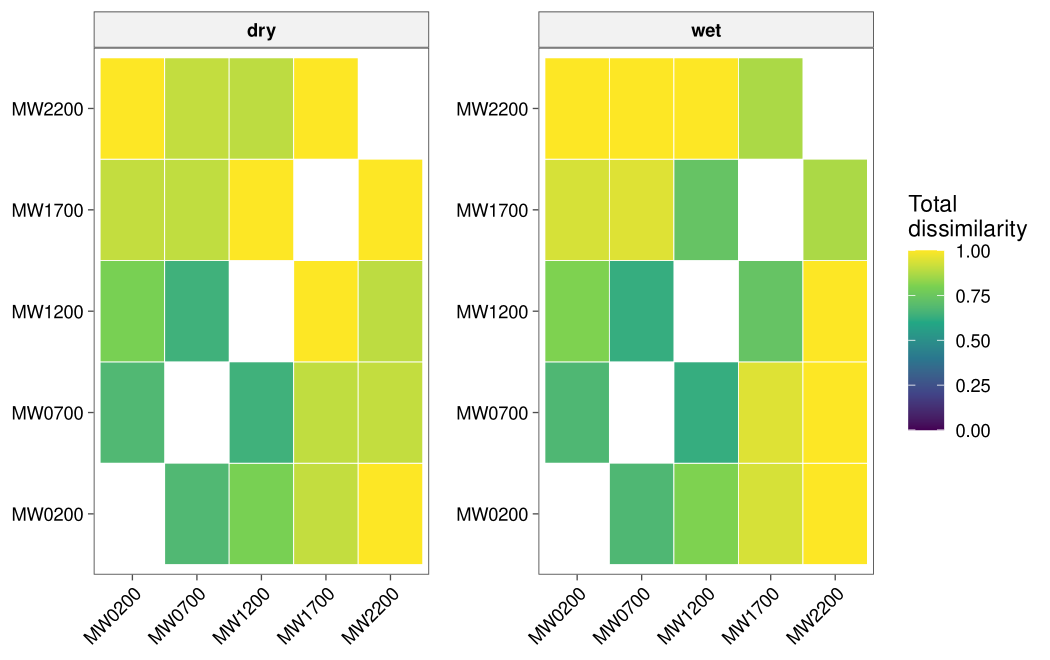
Total Sorensen dissimilarity between every pair of sites within each season.

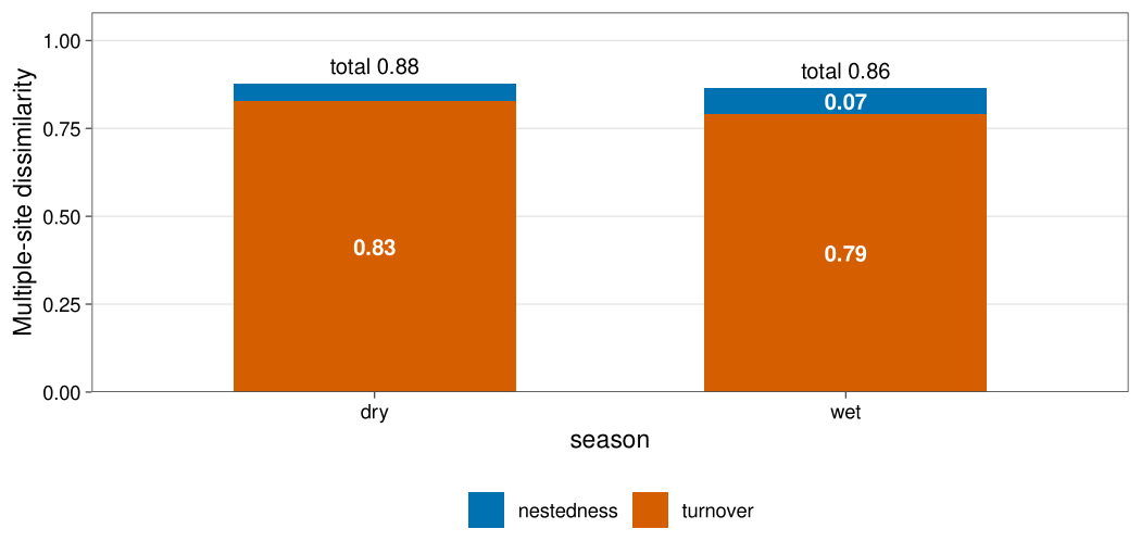
Multi-site beta partition

Multi-site Sorensen dissimilarity of each season split into turnover and nestedness.

Coverage-standardised beta diversity

Gamma, alpha and beta diversity of each season at 90% sample coverage, with 95% bootstrap intervals.

Distance decay

Pairwise total, turnover and nestedness dissimilarity against elevation difference, with quasibinomial (logit) trends that stay within 0-1.

Output tables

Example output of every main function on png_ants. Long tables show their first rows.

div_hill()

Observed Hill numbers: n occurrences, diversity of order q per site.

season	site	q	n	diversity
dry	MW0200	0	47	16.000
dry	MW0200	1	47	12.278
dry	MW0200	2	47	9.906
wet	MW0200	0	76	21.000
wet	MW0200	1	76	10.876
wet	MW0200	2	76	6.993
dry	MW0700	0	23	15.000
dry	MW0700	1	23	11.758

div_estimate()

Asymptotic estimates: observed and estimate Hill numbers with bootstrap se, lower and upper 95% limits.

season	site	q	observed	estimate	se	lower	upper
dry	MW0200	0	16.000	18.447	5.913	16.162	53.059
dry	MW0200	1	12.278	15.183	1.700	12.278	18.515
dry	MW0200	2	9.906	12.284	1.859	9.906	15.928
wet	MW0200	0	21.000	32.941	11.434	23.457	79.036
wet	MW0200	1	10.876	13.793	2.024	10.876	17.761
wet	MW0200	2	6.993	7.600	1.099	6.993	9.754
dry	MW0700	0	15.000	83.870	39.982	38.949	213.049
dry	MW0700	1	11.758	38.453	30.595	11.758	98.417

div_coverage()

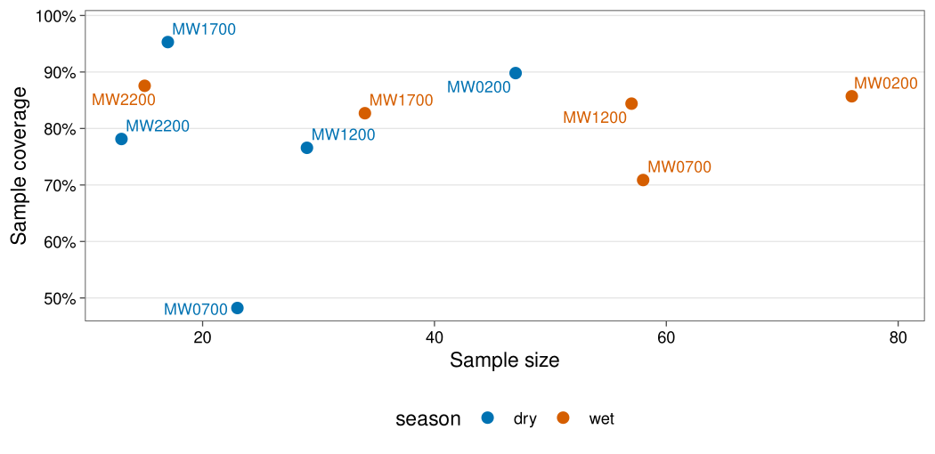
Sample coverage: n occurrences, s_obs observed species, f1 singletons, f2 doubletons and estimated coverage.

season	site	n	s_obs	f1	f2	coverage
dry	MW0200	47	16	5	5	0.898
wet	MW0200	76	21	11	5	0.857
dry	MW0700	23	15	12	1	0.482
wet	MW0700	58	28	17	3	0.709
dry	MW1200	29	13	7	3	0.766
wet	MW1200	57	20	9	3	0.844
dry	MW1700	17	5	1	2	0.953
wet	MW1700	34	10	6	2	0.827

div_rarefy()

Rarefaction and extrapolation: diversity of order q at sample size m, whether method is rarefaction, observed or extrapolation, the expected coverage, and lower and upper limits (NA when nboot = 0).

site	q	m	method	diversity	coverage	lower	upper
MW0200	0	1	rarefaction	1.000	0.132	NA	NA
MW0200	0	38	rarefaction	14.140	0.780	NA	NA
MW0200	0	75	rarefaction	20.855	0.855	NA	NA
MW0200	0	76	observed	21.000	0.857	NA	NA
MW0200	0	77	extrapolation	21.143	0.859	NA	NA
MW0200	0	102	extrapolation	24.211	0.895	NA	NA
MW0200	0	127	extrapolation	26.482	0.923	NA	NA
MW0200	0	152	extrapolation	28.162	0.943	NA	NA

div_standardise()

Coverage standardisation: diversity of order q at a common coverage for every site, with the matching sample size m, the method used, and bootstrap se, lower and upper limits.

season	site	q	m	method	coverage	diversity	se	lower	upper
dry	MW0200	0	11.646	rarefaction	0.565	7.963	0.458	7.067	8.860
dry	MW0200	1	11.646	rarefaction	0.565	7.099	0.513	6.093	8.105
dry	MW0200	2	11.646	rarefaction	0.565	6.236	0.534	5.189	7.283
wet	MW0200	0	45.094	rarefaction	0.796	15.651	1.415	12.877	18.425
wet	MW0200	1	45.094	rarefaction	0.796	9.570	1.071	7.471	11.668
wet	MW0200	2	45.094	rarefaction	0.796	6.630	0.816	5.031	8.228
dry	MW0700	0	46.000	extrapolation	0.565	25.975	5.306	15.575	36.374
dry	MW0700	1	46.000	extrapolation	0.565	17.858	6.141	5.821	29.895

beta_pair()

Pairwise beta diversity: Sorensen turnover (Simpson) and nestedness components, which sum to total dissimilarity.

season	site_1	site_2	turnover	nestedness	total
dry	MW0200	MW0700	0.667	0.011	0.677
dry	MW0200	MW1200	0.769	0.024	0.793
dry	MW0200	MW1700	0.800	0.105	0.905
dry	MW0200	MW2200	1.000	0.000	1.000
dry	MW0700	MW1200	0.615	0.027	0.643
dry	MW0700	MW1700	0.800	0.100	0.900
dry	MW0700	MW2200	0.833	0.071	0.905
dry	MW1200	MW1700	1.000	0.000	1.000

beta_multi()

Multi-site beta diversity: n_sites in each group with the multi-site turnover, nestedness and total.

season	n_sites	turnover	nestedness	total
dry	5	0.827	0.051	0.877
wet	5	0.790	0.074	0.864

beta_decay()

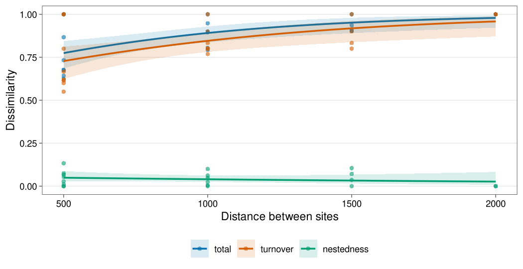
Distance decay: the pairwise components plus each site’s gradient_1 and gradient_2 values and their distance.

season	site_1	site_2	turnover	nestedness	total	gradient_1	gradient_2	distance
dry	MW0200	MW0700	0.667	0.011	0.677	200	700	500
dry	MW0200	MW1200	0.769	0.024	0.793	200	1200	1000
dry	MW0200	MW1700	0.800	0.105	0.905	200	1700	1500
dry	MW0200	MW2200	1.000	0.000	1.000	200	2200	2000
dry	MW0700	MW1200	0.615	0.027	0.643	700	1200	500
dry	MW0700	MW1700	0.800	0.100	0.900	700	1700	1000
dry	MW0700	MW2200	0.833	0.071	0.905	700	2200	1500
dry	MW1200	MW1700	1.000	0.000	1.000	1200	1700	500

beta_decay_model()

Distance-decay model of similarity: the fitted a and rate b, the half_distance over which similarity halves, the pseudo_r2, aic and a site-permutation p.value.

season	model	component	n_pairs	a	b	half_distance	pseudo_r2	aic	p.value
dry	exponential	total	10	0.257	0.001	924.159	0.143	-9.214	0.349
wet	exponential	total	10	0.897	0.002	293.331	0.694	-17.577	0.017

beta_hill_pair()

Pairwise Hill-number beta diversity of order q with the four normalised dissimilarities (first rows shown).

season	site_1	site_2	q	gamma	alpha	beta	dis_sorensen	dis_jaccard	dis_turnover_sorensen	dis_turnover_jaccard
dry	MW0200	MW0700	0	26	15.5	1.677	0.677	0.808	0.677	0.808
dry	MW0200	MW1200	0	26	14.5	1.793	0.793	0.885	0.793	0.885
dry	MW0200	MW1700	0	20	10.5	1.905	0.905	0.950	0.905	0.950
dry	MW0200	MW2200	0	22	11.0	2.000	1.000	1.000	1.000	1.000
dry	MW0700	MW1200	0	23	14.0	1.643	0.643	0.783	0.643	0.783
dry	MW0700	MW1700	0	19	10.0	1.900	0.900	0.947	0.900	0.947

beta_hill()

Coverage-standardised beta diversity: gamma, alpha and beta of order q at a common coverage, the sample sizes used (m_gamma, m_alpha) and four normalised dissimilarities.

season	q	coverage	m_gamma	m_alpha	gamma	alpha	beta	n_sites	dis_sorensen	dis_jaccard	dis_turnover_sorensen	dis_turnover_jaccard
dry	0	0.9	150.161	244.117	44.361	14.476	3.064	5	0.516	0.842	0.516	0.842
dry	1	0.9	150.161	244.117	30.995	9.929	3.122	5	0.707	0.707	0.530	0.850
dry	2	0.9	150.161	244.117	23.324	6.968	3.347	5	0.877	0.587	0.587	0.877
wet	0	0.9	259.764	480.767	64.058	23.502	2.726	5	0.431	0.791	0.431	0.791
wet	1	0.9	259.764	480.767	35.366	12.345	2.865	5	0.654	0.654	0.466	0.814
wet	2	0.9	259.764	480.767	21.377	7.081	3.019	5	0.836	0.505	0.505	0.836

beta_welch()

Welch-type PERMANOVA (W*d), robust to unequal dispersion: the statistic, the numbers of groups and sites, and the permutation p.value.

statistic	n_groups	n_sites	p.value
1.29	2	20	0.179

References

• Chao, A. et al. (2014). Rarefaction and extrapolation with Hill numbers. Ecological Monographs, 84, 45-67.
• Chao, A. and Jost, L. (2012). Coverage-based rarefaction and extrapolation. Ecology, 93, 2533-2547.
• Baselga, A. (2010). Partitioning the turnover and nestedness components of beta diversity. Global Ecology and Biogeography, 19, 134-143.
• Blanchet, F. G., Legendre, P. and Borcard, D. (2008). Forward selection of explanatory variables. Ecology, 89, 2623-2632.
• Carmona, C. P. et al. (2019). Trait probability density (TPD): measuring functional diversity across scales based on TPD with R. Ecology, 100, e02876.
• Chao, A., Chiu, C.-H. and Jost, L. (2014). Unifying species diversity, phylogenetic diversity, functional diversity, and related similarity and differentiation measures through Hill numbers. Annual Review of Ecology, Evolution, and Systematics, 45, 297-324.
• Chao, A. et al. (2019). An attribute-diversity approach to functional diversity, functional beta diversity, and related (dis)similarity measures. Ecological Monographs, 89, e01343.
• Chao, A. et al. (2023). Rarefaction and extrapolation with beta diversity under a framework of Hill numbers: the iNEXT.beta3D standardization. Ecological Monographs, 93, e1588.
• de Bello, F. et al. (2021). Handbook of Trait-Based Ecology: From Theory to R Tools. Cambridge University Press.
• Hamidi, B. et al. (2019). Wd-test: robust distance-based multivariate analysis of variance. Microbiome*, 7, 51.
• Gómez-Rodríguez, C. and Baselga, A. (2018). Variation among European beetle taxa in patterns of distance decay of similarity suggests a major role of dispersal processes. Ecography, 41, 1825-1834.
• Moses, J. et al. (2023). Nutrient use by tropical ant communities varies among three extensive elevational gradients: a cross-continental comparison. Global Ecology and Biogeography, 32, 2212-2229.
• Nekola, J. C. and White, P. S. (1999). The distance decay of similarity in biogeography and ecology. Journal of Biogeography, 26, 867-878.
• Zeleny, D. (2018). Which results of the standard test for community-weighted mean approach are too optimistic? Journal of Vegetation Science, 29, 953-966.

Licence

MIT © Jimmy Moses