Diversity estimates are often the response in a model of environmental drivers. Two things matter: the estimates should be comparable (equal coverage or asymptotic), and their uncertainty should carry through to the model. tidydiversity results are tidy tibbles, so this takes a few lines.
library(tidydiversity)
library(dplyr)
library(ggplot2)
set.seed(2026)
sites <- distinct(png_ants, site, elevation)
Model-ready estimates
tidy() renames columns to the broom conventions and adds
an inverse-variance weight; add_site_data()
joins covariates that are constant within each site.
est <- div_standardise(png_ants,
  q = c(0, 1, 2), .by = season,
  nboot = 200
) |>
  tidy() |>
  add_site_data(sites)
est
#> # A tibble: 30 x 12
#>    season site       q     m method        coverage estimate std.error conf.low
#>    <chr>  <chr>  <dbl> <dbl> <chr>            <dbl>    <dbl>     <dbl>    <dbl>
#>  1 dry    MW0200     0  11.6 rarefaction      0.565     7.96     0.489     7.00
#>  2 dry    MW0200     1  11.6 rarefaction      0.565     7.10     0.549     6.02
#>  3 dry    MW0200     2  11.6 rarefaction      0.565     6.24     0.563     5.13
#>  4 wet    MW0200     0  45.1 rarefaction      0.796    15.7      1.55     12.6
#>  5 wet    MW0200     1  45.1 rarefaction      0.796     9.57     1.24      7.14
#>  6 wet    MW0200     2  45.1 rarefaction      0.796     6.63     0.926     4.82
#>  7 dry    MW0700     0  46.0 extrapolation    0.565    26.0      4.76     16.6
#>  8 dry    MW0700     1  46.0 extrapolation    0.565    17.9      5.06      7.95
#>  9 dry    MW0700     2  46.0 extrapolation    0.565    10.5      4.64      1.42
#> 10 wet    MW0700     0 116   extrapolation    0.796    42.2      6.21     30.1
#> # i 20 more rows
#> # i 3 more variables: conf.high <dbl>, weight <dbl>, elevation <int>
Approaches
Inverse-variance weights give less influence to imprecise estimates.
# A site with one species has a zero standard error and no weight
shannon <- filter(est, q == 1, !is.na(weight))
fit_lm <- lm(estimate ~ elevation + I(elevation^2) + season,
  data = shannon, weights = weight
)
broom::tidy(fit_lm, conf.int = TRUE)
#> # A tibble: 4 x 7
#>   term              estimate  std.error statistic p.value    conf.low  conf.high
#>   <chr>                <dbl>      <dbl>     <dbl>   <dbl>       <dbl>      <dbl>
#> 1 (Intercept)     8.61       2.23           3.87  0.00830  3.16          1.41e+1
#> 2 elevation      -0.00557    0.00376       -1.48  0.189   -0.0148        3.63e-3
#> 3 I(elevation^2)  0.00000117 0.00000154     0.760 0.476   -0.00000260    4.95e-6
#> 4 seasonwet       2.42       1.72           1.40  0.210   -1.80          6.64e+0
Each elevation band was sampled in both seasons, so sites are repeated. Add a random effect for site with lme4 (or glmmTMB, which takes the same formula).
fit_mm <- lme4::lmer(estimate ~ elevation + season + (1 | site),
  data = shannon, weights = weight / mean(weight)
)
summary(fit_mm)$coefficients
#>                 Estimate  Std. Error   t value
#> (Intercept)  8.335239972 1.936638262  4.303974
#> elevation   -0.002897246 0.001183797 -2.447418
#> seasonwet    2.126186442 1.391201962  1.528309
mgcv fits a smooth response along the gradient.
fit_gam <- mgcv::gam(estimate ~ s(elevation, k = 4) + season,
  data = shannon, weights = weight / mean(weight), method = "REML"
)
summary(fit_gam)$s.table
#>                  edf  Ref.df        F    p-value
#> s(elevation) 1.00008 1.00016 8.487165 0.02254615
grid <- tidyr::expand_grid(
  elevation = seq(200, 2200, by = 20),
  season = c("wet", "dry")
)
pred <- predict(fit_gam, grid, se.fit = TRUE)
grid$fit <- pred$fit
grid$se <- pred$se.fit
ggplot(grid, aes(elevation, fit, colour = season, fill = season)) +
  geom_ribbon(aes(ymin = fit - 1.96 * se, ymax = fit + 1.96 * se),
    alpha = 0.2, colour = NA
  ) +
  geom_line() +
  geom_pointrange(aes(y = estimate, ymin = conf.low, ymax = conf.high),
    data = shannon
  ) +
  scale_colour_tidydiversity() +
  scale_fill_tidydiversity() +
  labs(
    x = "Elevation (m)",
    y = "Shannon diversity (effective number of species)",
    colour = NULL, fill = NULL
  ) +
  theme_tidydiversity()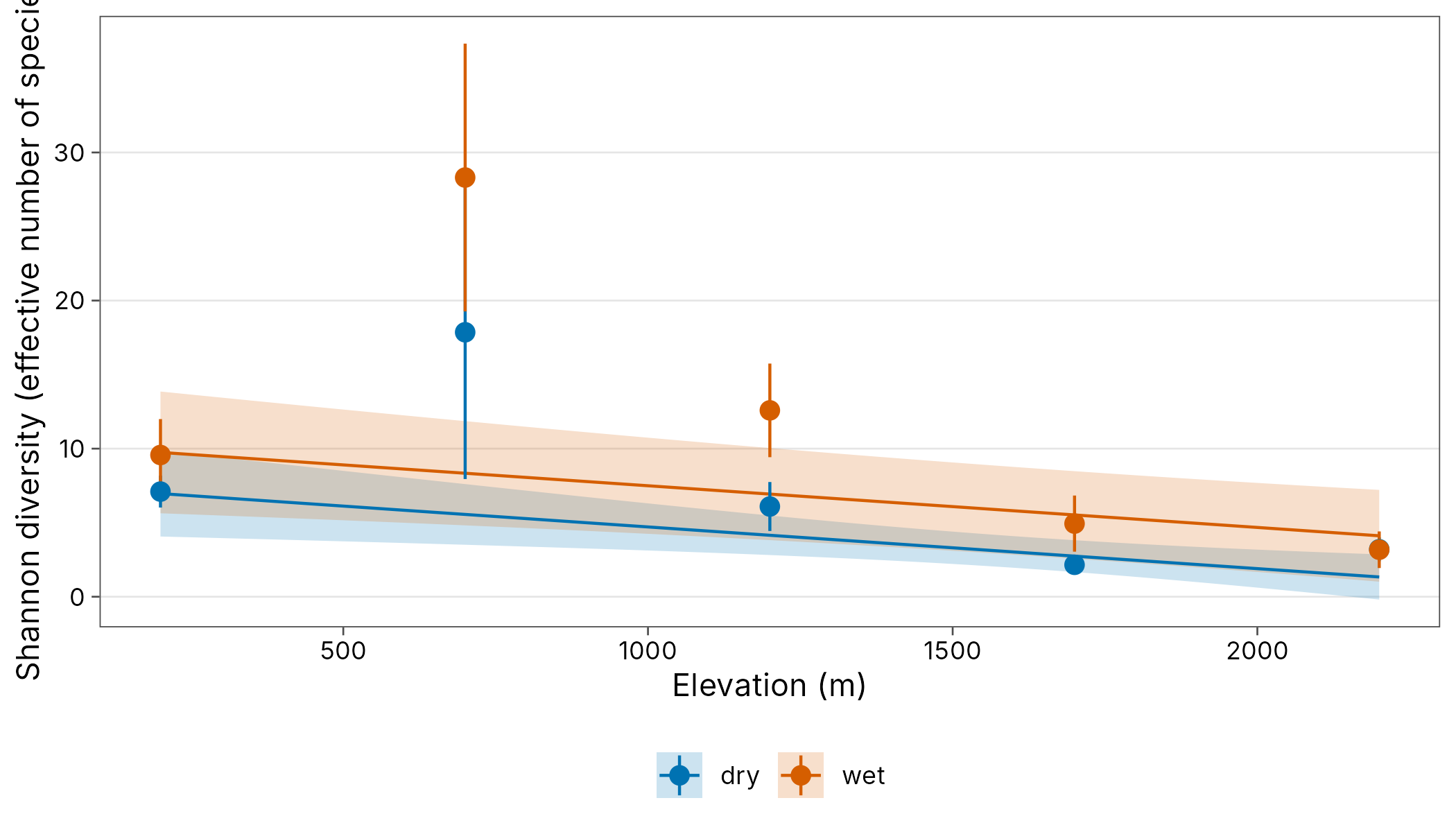
Observed richness is a count, but it depends on sampling effort. Model standardised richness with a Gamma GLM (positive, continuous), or observed richness with a Poisson GLM and log sample size as an offset.
rich <- filter(est, q == 0, !is.na(weight))
broom::tidy(glm(estimate ~ elevation + season,
  data = rich,
  family = Gamma(link = "log"), weights = weight / mean(weight)
))
#> # A tibble: 3 x 5
#>   term         estimate std.error statistic p.value
#>   <chr>           <dbl>     <dbl>     <dbl>   <dbl>
#> 1 (Intercept)  2.10      0.440         4.78 0.00200
#> 2 elevation   -0.000597  0.000259     -2.31 0.0544
#> 3 seasonwet    0.822     0.498         1.65 0.143
obs <- div_hill(png_ants, q = 0, .by = season) |> add_site_data(sites)
broom::tidy(glm(diversity ~ elevation + season + offset(log(n)),
  data = obs, family = poisson
))
#> # A tibble: 3 x 5
#>   term          estimate std.error statistic    p.value
#>   <chr>            <dbl>     <dbl>     <dbl>      <dbl>
#> 1 (Intercept) -0.874      0.181       -4.81  0.00000148
#> 2 elevation    0.0000230  0.000131     0.175 0.861
#> 3 seasonwet   -0.197      0.173       -1.14  0.256
Propagating uncertainty with bootstrap draws
Weights use only the standard error. div_boot() returns
the bootstrap replicates themselves, so the whole model can be refitted
to each replicate and the spread of the coefficients includes the
estimation uncertainty in the response.
draws <- div_boot(png_ants,
  q = 1, type = "standardised", .by = season,
  coverage = 0.9, nboot = 200
) |>
  add_site_data(sites)
draws
#> # A tibble: 2,000 x 7
#>    season site       q     m .draw diversity elevation
#>    <chr>  <chr>  <dbl> <dbl> <int>     <dbl>     <int>
#>  1 dry    MW0200     1  47.5     1      8.01       200
#>  2 dry    MW0200     1  47.5     2     11.3        200
#>  3 dry    MW0200     1  47.5     3      9.80       200
#>  4 dry    MW0200     1  47.5     4      8.38       200
#>  5 dry    MW0200     1  47.5     5      9.94       200
#>  6 dry    MW0200     1  47.5     6      8.98       200
#>  7 dry    MW0200     1  47.5     7     12.8        200
#>  8 dry    MW0200     1  47.5     8     12.4        200
#>  9 dry    MW0200     1  47.5     9     13.2        200
#> 10 dry    MW0200     1  47.5    10     12.2        200
#> # i 1,990 more rows

slopes <- draws |>
  group_by(.draw) |>
  group_modify(\(d, key) {
    broom::tidy(lm(diversity ~ elevation + season, data = d))
  }) |>
  ungroup() |>
  filter(term == "elevation")
quantile(slopes$estimate, c(0.025, 0.5, 0.975))
#>         2.5%          50%        97.5%
#> -0.011902670 -0.007785796 -0.005202705
ggplot(slopes, aes(estimate * 100)) +
  geom_histogram(bins = 30, fill = plot_palette(1)) +
  geom_vline(xintercept = 0, linetype = "dashed") +
  labs(x = "Change in Shannon diversity per 100 m", y = "Bootstrap draws") +
  theme_tidydiversity()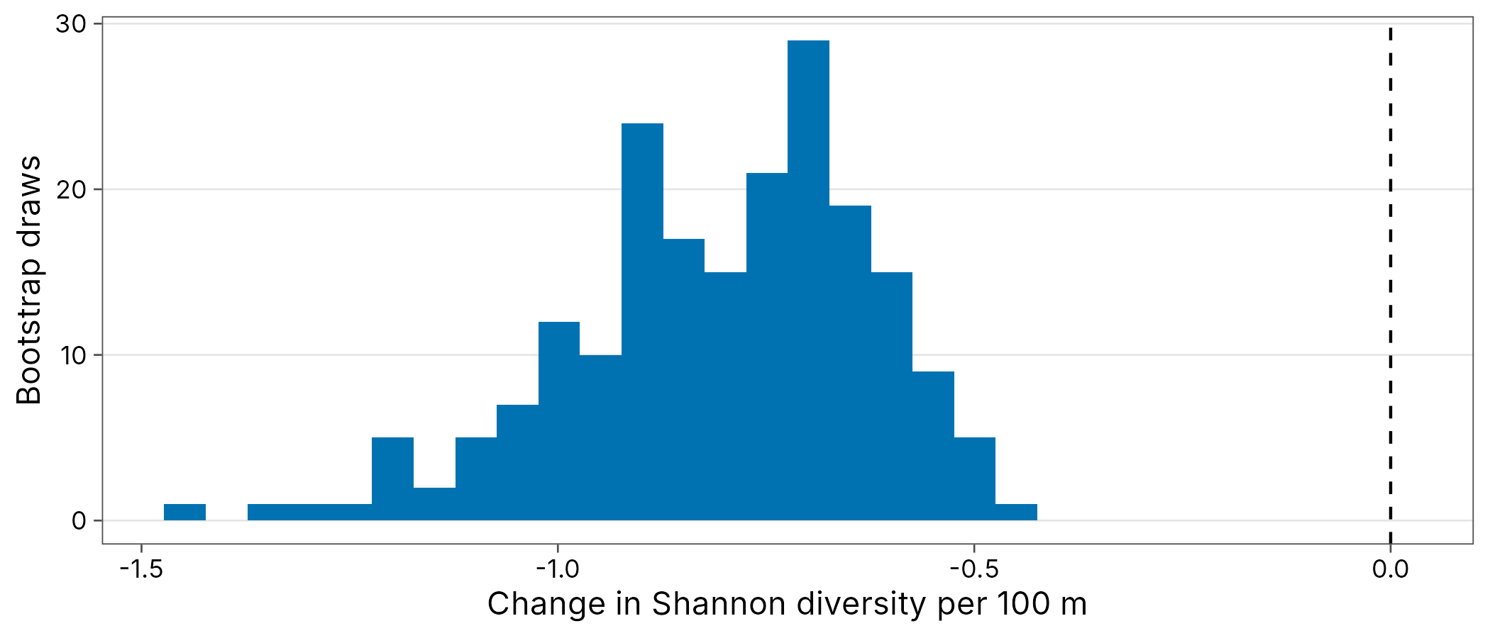
Beta diversity
Distance decay
beta_decay() gives one row per pair of sites with the
distance along one or more gradients. Several columns give Euclidean
distance.
decay <- beta_decay(png_ants, elevation, .by = season)
broom::tidy(lm(turnover ~ distance + season, data = decay))
#> # A tibble: 3 x 5
#>   term         estimate std.error statistic      p.value
#>   <chr>           <dbl>     <dbl>     <dbl>        <dbl>
#> 1 (Intercept)  0.664    0.0723        9.18  0.0000000531
#> 2 distance     0.000168 0.0000590     2.85  0.0110
#> 3 seasonwet   -0.0149   0.0590       -0.252 0.804
Pairs are not independent, so test the relationship with a Mantel test rather than the lm p-values.
wet <- filter(png_ants, season == "wet")
d_beta <- beta_dist(beta_pair(wet), "turnover")
d_elev <- dist(distinct(wet, site, elevation)$elevation)
vegan::mantel(d_beta, d_elev, permutations = 999)
#> 'nperm' >= set of all permutations: complete enumeration.
#> Set of permutations < 'minperm'. Generating entire set.
#>
#> Mantel statistic based on Pearson's product-moment correlation
#>
#> Call:
#> vegan::mantel(xdis = d_beta, ydis = d_elev, permutations = 999)
#>
#> Mantel statistic r: 0.8064
#>       Significance: 0.016667
#>
#> Upper quantiles of permutations (null model):
#>   90%   95% 97.5%   99%
#> 0.443 0.515 0.522 0.655
#> Permutation: free
#> Number of permutations: 119
PERMANOVA and ordination
# One sampling unit per elevation band and season
units <- mutate(png_ants, unit = paste(site, season))
bray <- beta_dist(beta_pair(units, site = unit, index = "bray"))
unit_data <- distinct(units, unit, site, season, elevation)
unit_data <- unit_data[match(labels(bray), unit_data$unit), ]
vegan::adonis2(bray ~ elevation + season,
  data = unit_data,
  permutations = 999
)
#> Permutation test for adonis under reduced model
#> Permutation: free
#> Number of permutations: 999
#>
#> vegan::adonis2(formula = bray ~ elevation + season, data = unit_data, permutations = 999)
#>          Df SumOfSqs      R2      F Pr(>F)
#> Model     2   1.1156 0.30648 1.5467  0.055 .
#> Residual  7   2.5244 0.69352
#> Total     9   3.6400 1.00000
#> ---
#> Signif. codes:  0 '***' 0.001 '**' 0.01 '*' 0.05 '.' 0.1 ' ' 1
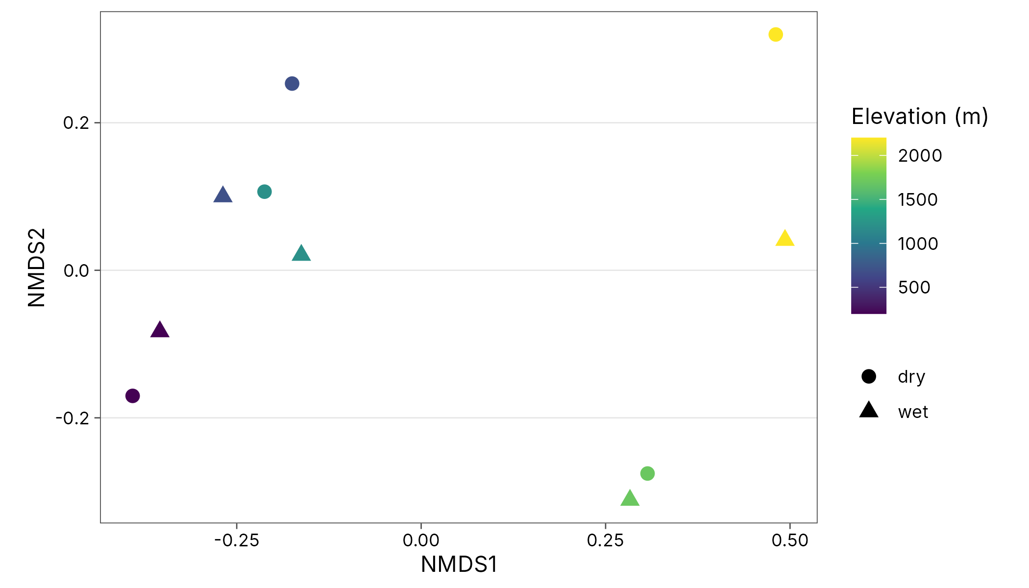
nmds <- vegan::metaMDS(bray, trace = FALSE)
bind_cols(unit_data, as.data.frame(vegan::scores(nmds))) |>
  ggplot(aes(NMDS1, NMDS2, colour = elevation, shape = season)) +
  geom_point(size = 3) +
  scale_colour_viridis_c() +
  coord_equal() +
  labs(colour = "Elevation (m)", shape = NULL) +
  theme_tidydiversity(legend_position = "right")