Case study: forest birds and North American bird communities

Two bird datasets cover the alpha and beta parts of the workflow.

Sources and licences.

• bird in iNEXT (GPL-3 or later): counts of 41 species at a northern and a southern site in a Taiwanese forest, from Chao et al. (2014).
• bbs1980 and bbs2000 in betapart (GPL-2 or later): presence or absence of 569 breeding bird species in 49 states of the contiguous USA, from the North American Breeding Bird Survey (Sauer et al. 2011), as used by Baselga and Orme (2012).

Both are loaded from their packages at run time and are not redistributed with tidydiversity.

library(tidydiversity)
library(dplyr)
library(ggplot2)
set.seed(2026)

Alpha diversity at two forest sites

data(bird, package = "iNEXT")
birds <- tibble::tibble(
  species = sprintf("sp%02d", seq_len(nrow(bird))),
  North = bird$North.site,
  South = bird$South.site
) |>
  tidyr::pivot_longer(-species,
    names_to = "site",
    values_to = "abundance"
  ) |>
  as_community()
div_coverage(birds)
#> # A tibble: 2 x 6
#>   site      n s_obs    f1    f2 coverage
#>   <chr> <int> <int> <int> <int>    <dbl>
#> 1 North   202    27     6     4    0.970
#> 2 South   307    38     5     6    0.984

Asymptotic estimates

These match iNEXT::iNEXT() to numerical precision (see the package tests). The richness interval is the asymmetric log-normal interval of Chao (1987), so it never falls below the observed richness.

est <- div_estimate(birds, nboot = 200)
div_table(est, digits = 1, output = "kable")

site	Order q	Observed	Estimate [95% CI]
North	0	27.0	31.5 [27.4, 72.5]
North	1	16.5	18.0 [16.5, 20.4]
North	2	11.8	12.5 [11.8, 14.8]
South	0	38.0	40.1 [38.1, 83.4]
South	1	25.4	27.3 [25.4, 29.9]
South	2	19.6	20.9 [19.6, 23.9]

autoplot(est)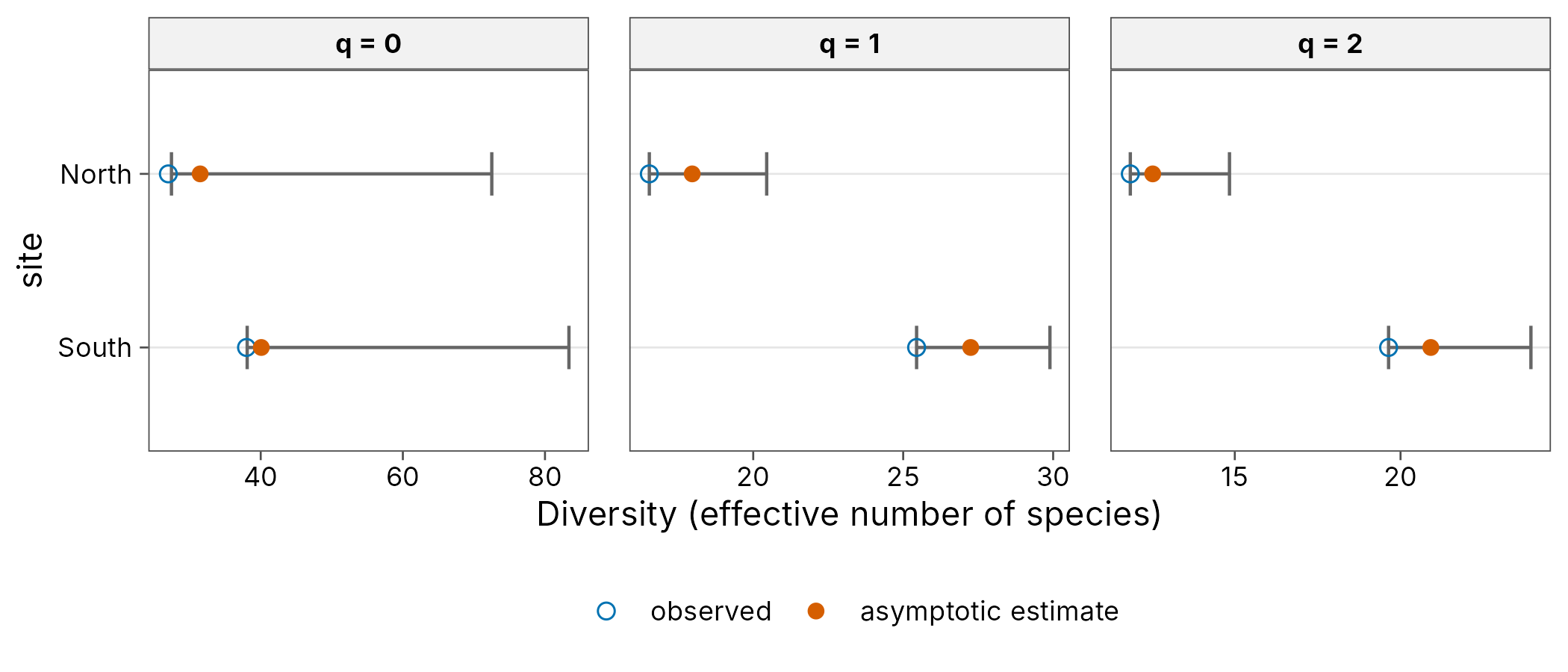

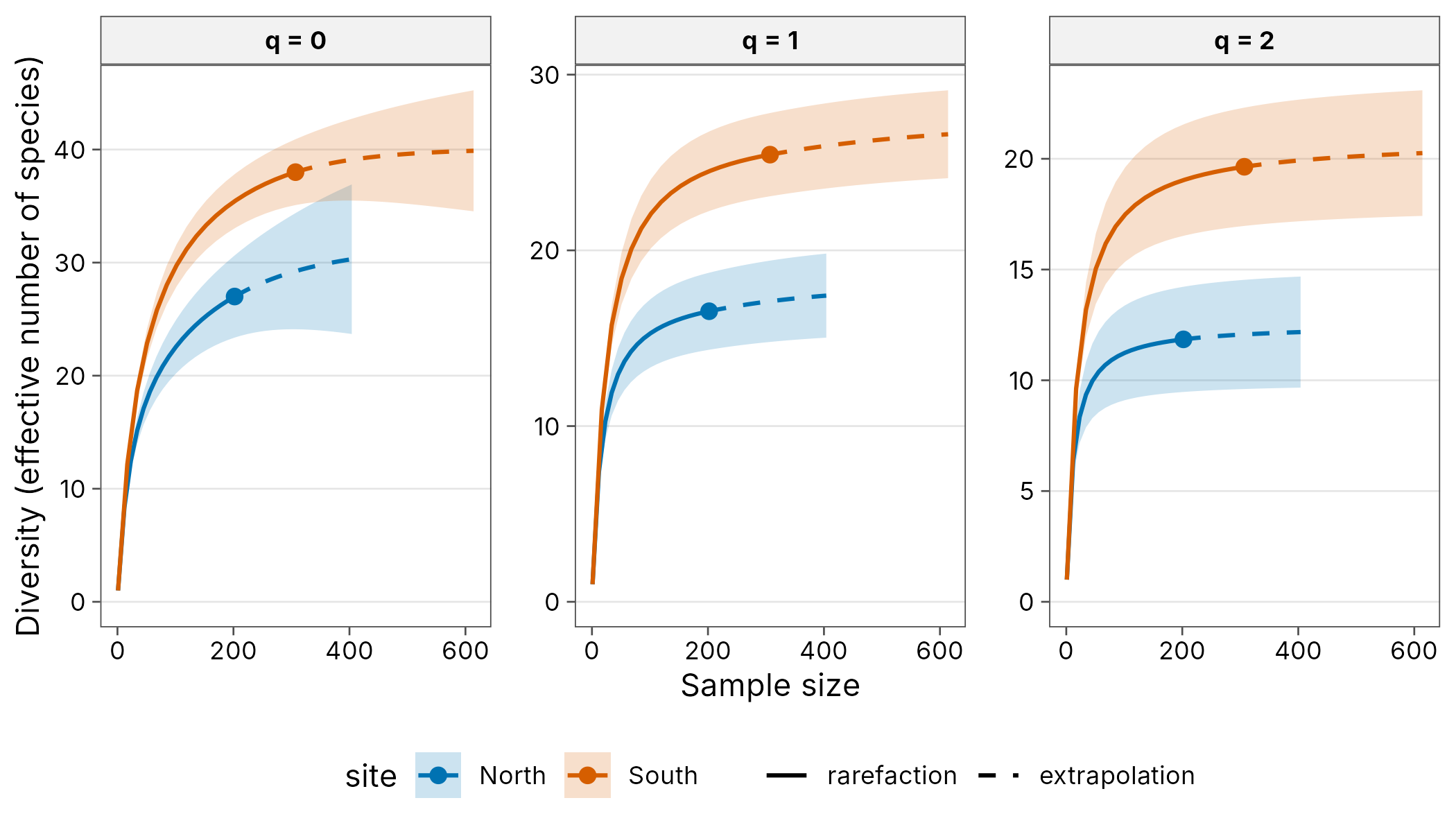
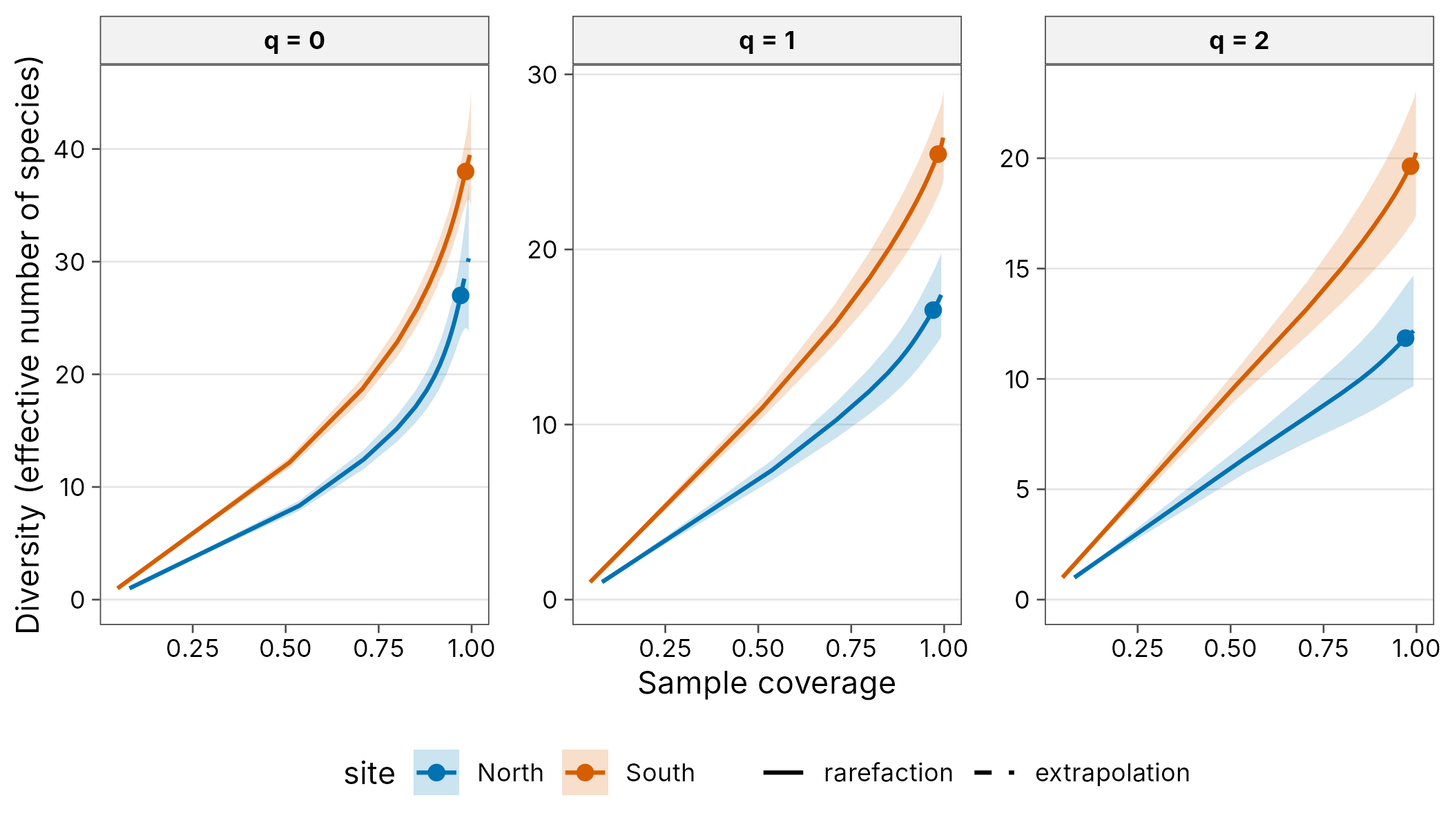
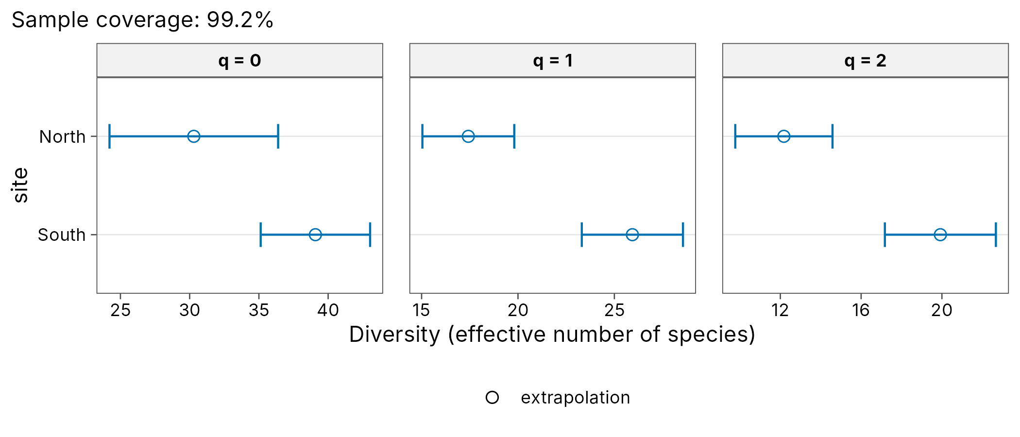
Curves

curves <- div_rarefy(birds, nboot = 200)
autoplot(curves)

autoplot(curves, x = "coverage")

Comparing at equal coverage

std <- div_standardise(birds, nboot = 200)
autoplot(std)

Beta diversity across the USA

data(bbsData, package = "betapart")
to_long <- function(m, year) {
  community_long(
    tibble::as_tibble(m, rownames = "site") |> mutate(year = year),
    cols = -c(site, year)
  )
}
bbs <- bind_rows(to_long(bbs1980, 1980), to_long(bbs2000, 2000))
bbs
#> # A community: 49 sites, 569 species, 16,582 individuals
#>     year site  species abundance
#>    <dbl> <chr> <chr>       <int>
#>  1  1980 AK    100             1
#>  2  1980 AK    110             1
#>  3  1980 AK    1230            1
#>  4  1980 AK    1290            1
#>  5  1980 AK    1300            1
#>  6  1980 AK    1320            1
#>  7  1980 AK    1350            1
#>  8  1980 AK    1370            1
#>  9  1980 AK    1390            1
#> 10  1980 AK    140             1
#> # i 16,572 more rows

Multiple-site partitions

Sorensen dissimilarity among all 49 states, split into turnover (replacement of species) and nestedness (loss of species).

multi <- beta_multi(bbs, .by = year)
multi
#> # A tibble: 2 x 5
#>    year n_sites turnover nestedness total
#>   <dbl>   <int>    <dbl>      <dbl> <dbl>
#> 1  1980      49    0.886     0.0325 0.918
#> 2  2000      49    0.878     0.0368 0.915
autoplot(multi, xlab = "Year")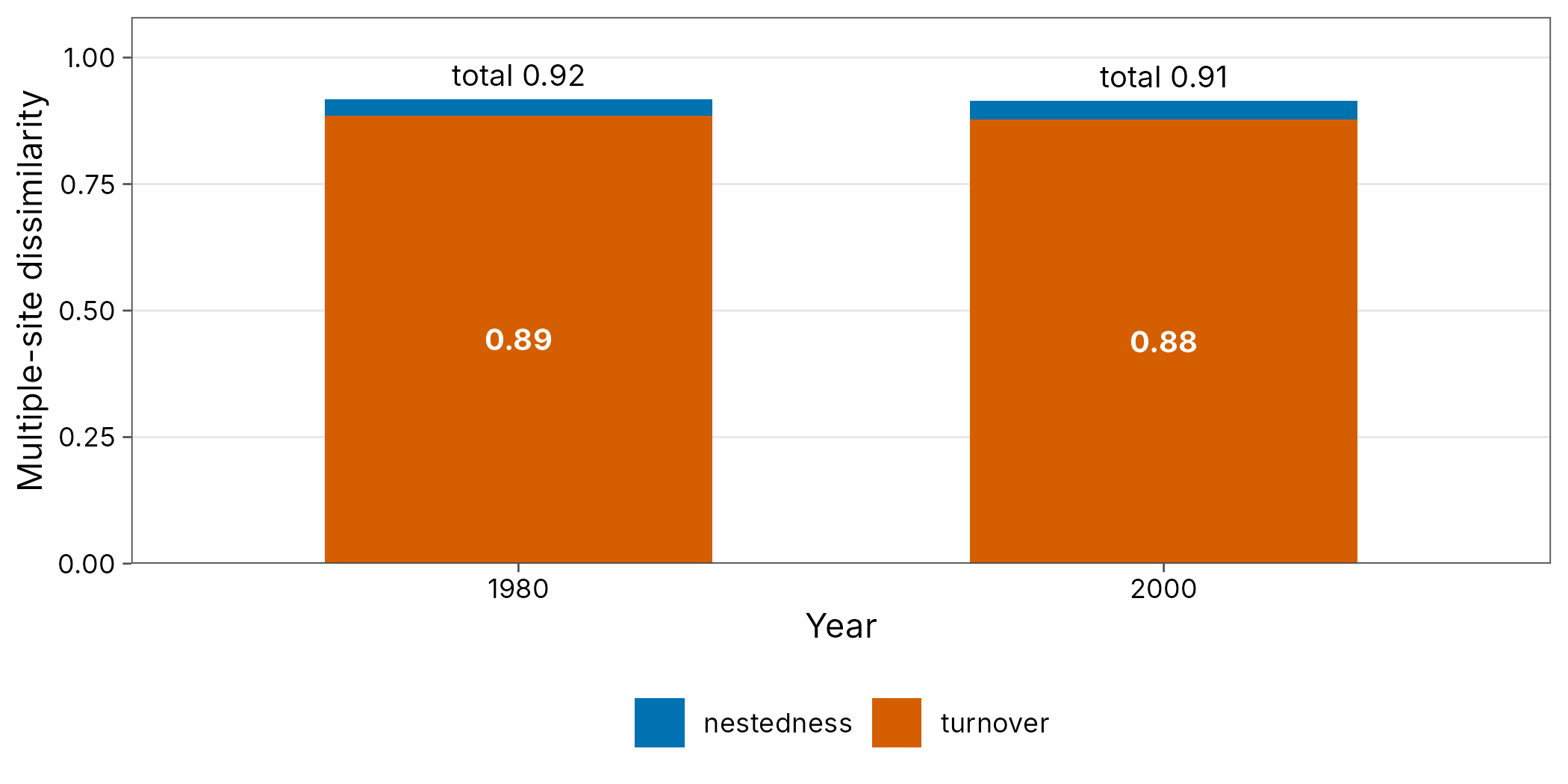

Change in each state

Pairing each state with itself 20 years later gives the temporal beta diversity of each state.

temporal <- bbs |>
  mutate(site = paste(site, year)) |>
  beta_pair() |>
  filter(sub(" .*", "", site_1) == sub(" .*", "", site_2)) |>
  mutate(state = sub(" .*", "", site_1))
temporal |>
  tidyr::pivot_longer(c(turnover, nestedness), names_to = "component") |>
  ggplot(aes(value, fill = component)) +
  geom_histogram(bins = 20, position = "identity", alpha = 0.7) +
  scale_fill_tidydiversity() +
  labs(
    x = "Dissimilarity between 1980 and 2000", y = "Number of states",
    fill = NULL
  ) +
  theme_tidydiversity()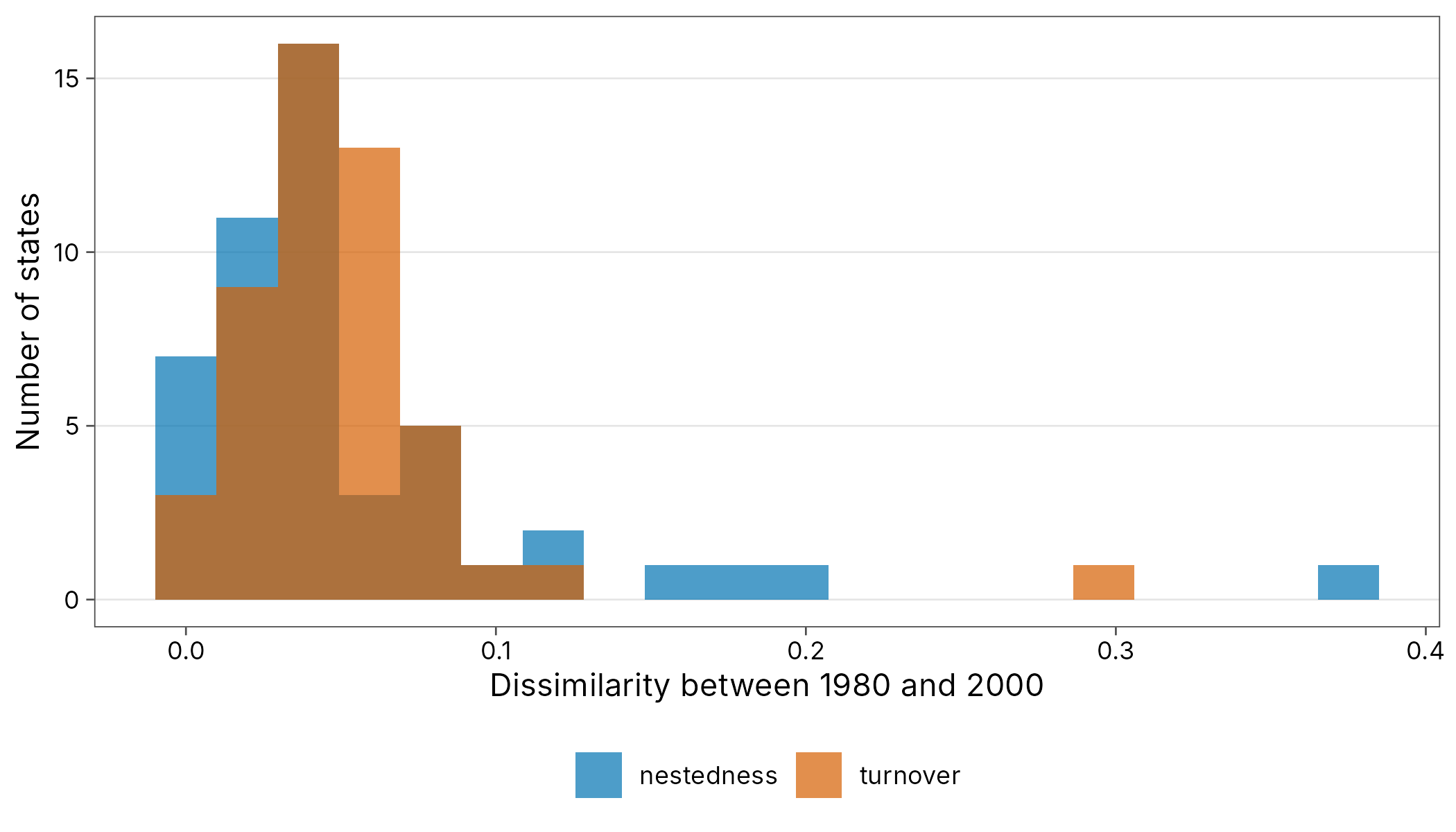

References

Baselga, A. and Orme, C. D. L. (2012). betapart: an R package for the study of beta diversity. Methods in Ecology and Evolution 3: 808-812.

Chao, A. (1987). Estimating the population size for capture-recapture data with unequal catchability. Biometrics 43: 783-791.

Chao, A., Gotelli, N. J., Hsieh, T. C., et al. (2014). Rarefaction and extrapolation with Hill numbers. Ecological Monographs 84: 45-67.

Sauer, J. R., Hines, J. E., Fallon, J. E., et al. (2011). The North American Breeding Bird Survey, results and analysis 1966-2009. USGS Patuxent Wildlife Research Center.