Real-world tutorials

Seven tutorials run the full workflow (tidy the data, check completeness, draw curves, standardise, model against covariates, partition beta diversity and report) on published, properly cited datasets. Each tab gives a short preview; follow the link for the whole analysis.

library(tidydiversity)
library(dplyr)
library(ggplot2)
set.seed(1)

Papua New Guinea

• Ants
• Frogs
• Butterflies

Ground ants at baits along Mt Wilhelm (png_ants; Moses et al. 2023) and tree-nesting ants in three forest plots (png_tree_ants; Plowman et al. 2020). Full tutorial.

div_estimate(png_tree_ants, abundance = nests, nboot = 50) |>
  autoplot()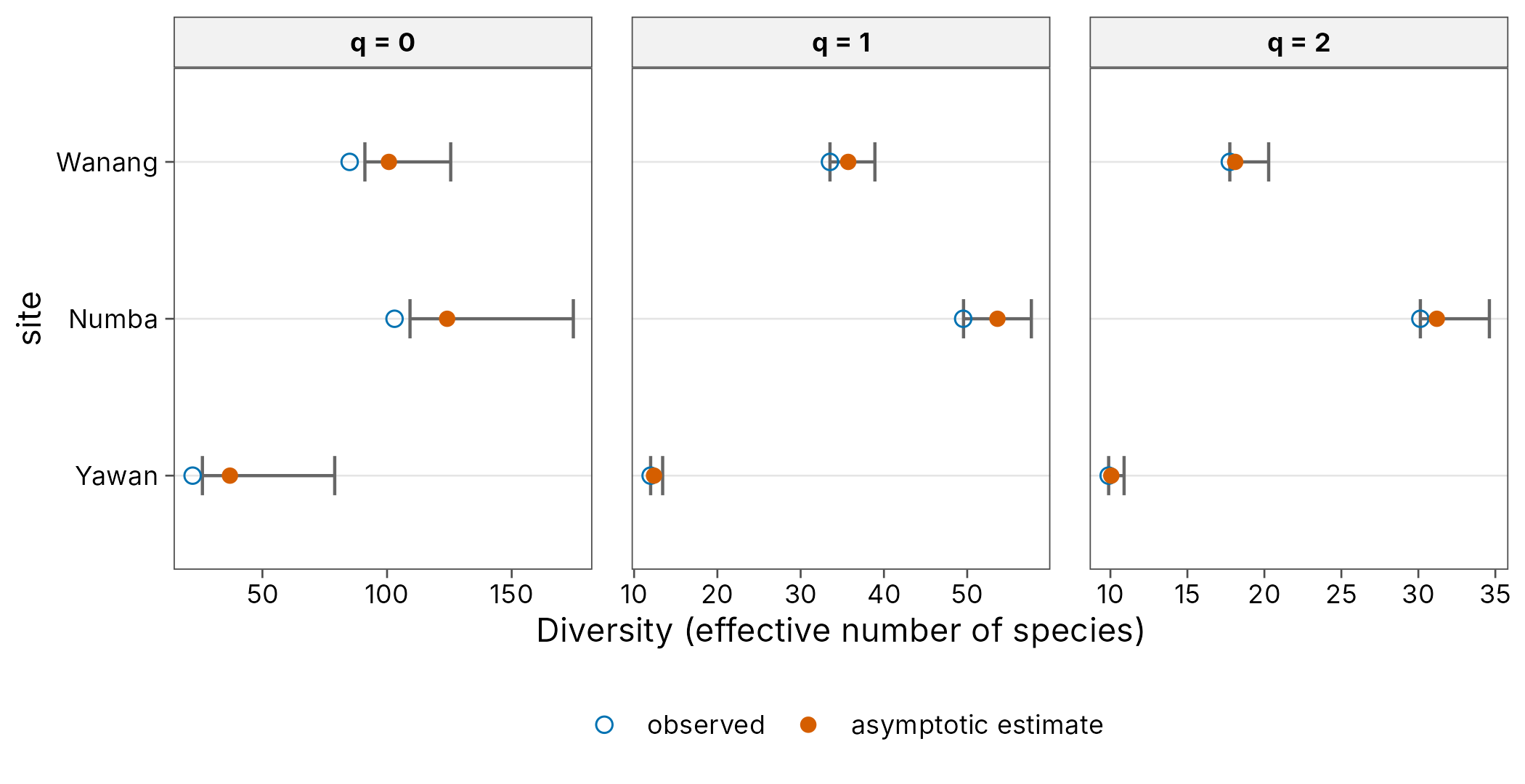

Frogs at eight elevations from 200 to 3700 m on Mt Wilhelm (png_frogs; Dahl et al. 2024). Full tutorial.

beta_decay(png_frogs, gradient = elevation) |>
  autoplot()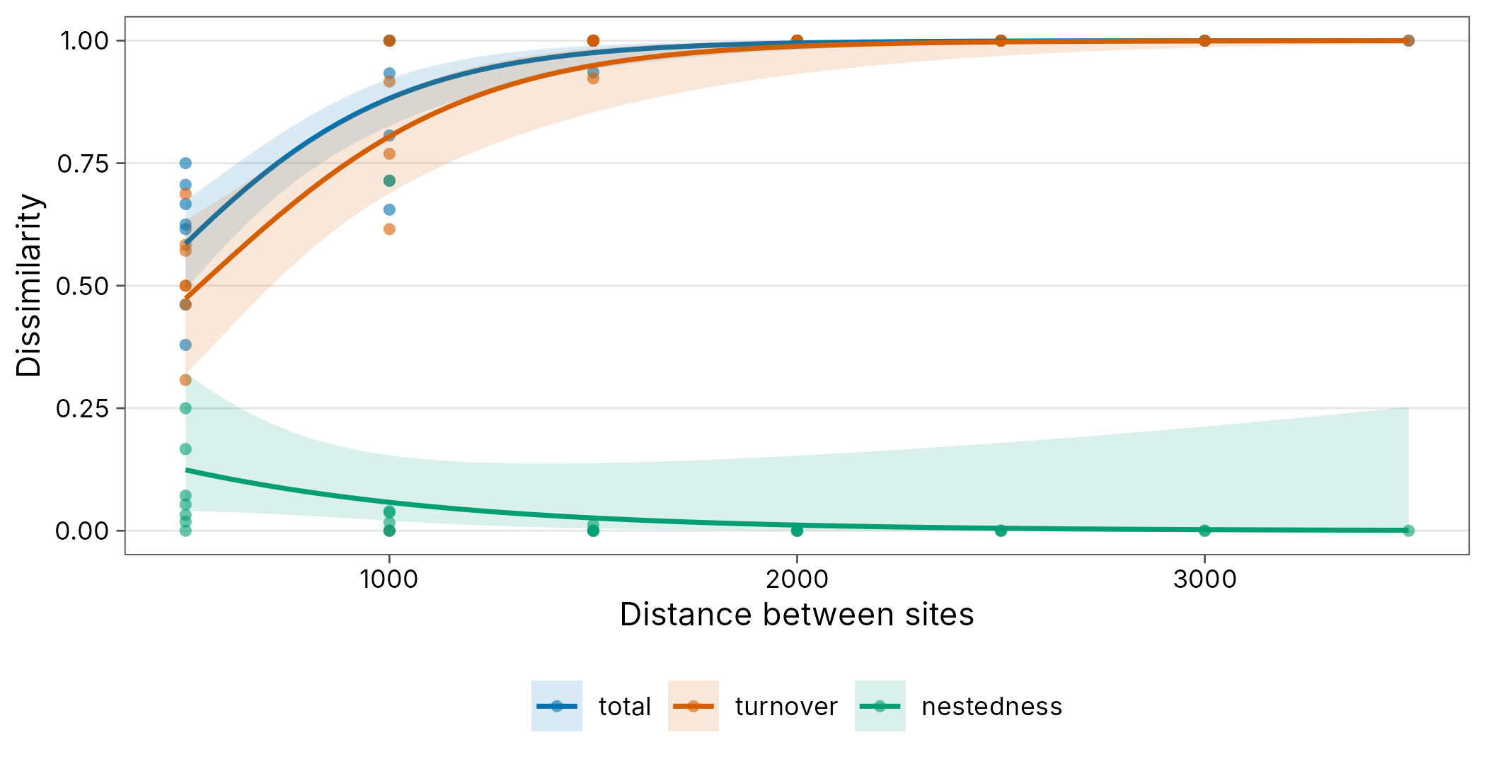

Three years of butterfly monitoring in the Wanang forest plot (wanang_butterflies; Luk et al. 2019). Full tutorial.

wanang_butterflies |>
  mutate(site = paste("Year", year)) |>
  div_rarefy(q = 0, knots = 30) |>
  autoplot()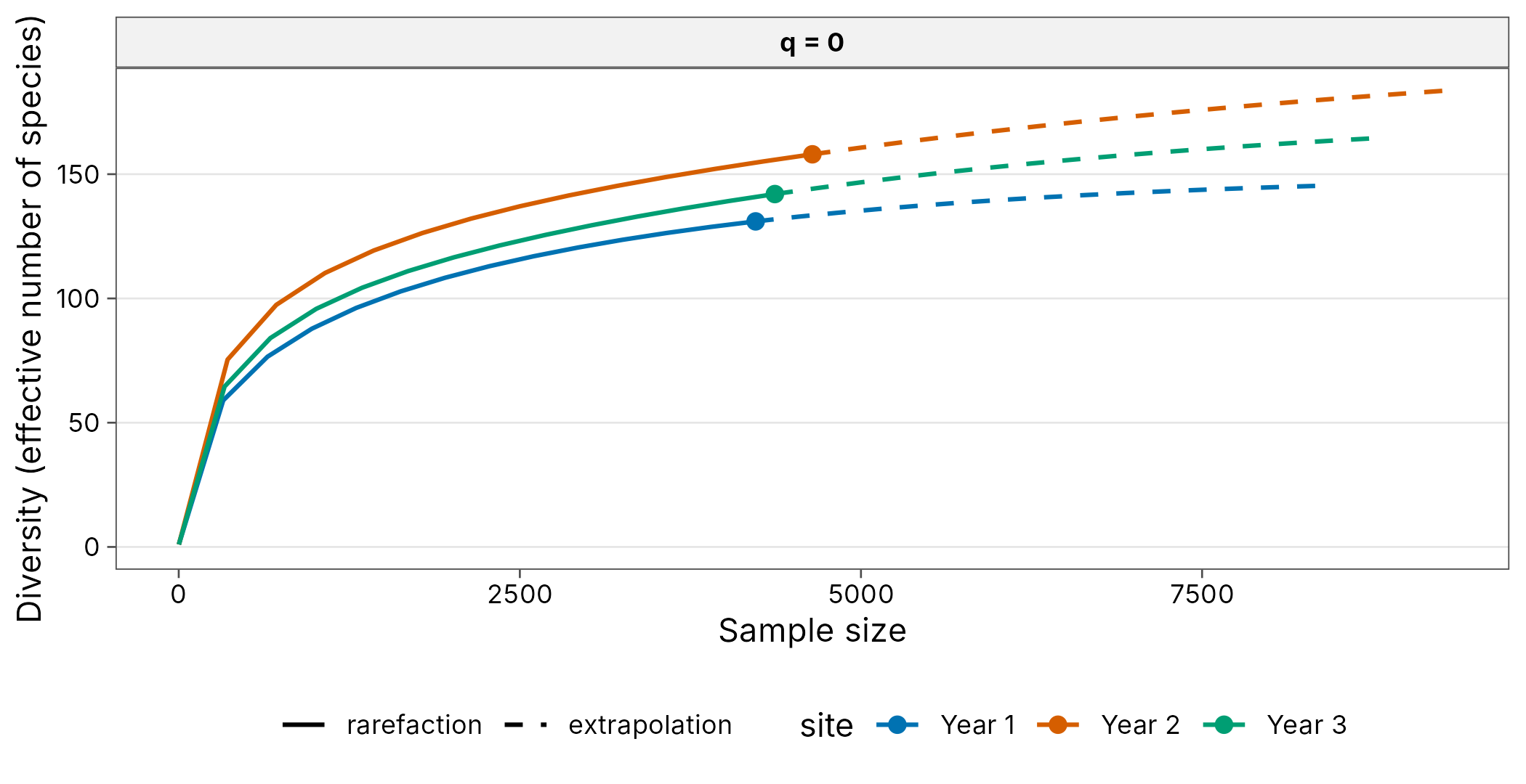

Other regions

• Insects
• Mammals
• Birds
• Plants

Caddisflies at a light trap on the Rhône (ade4 trichometeo), 49 nights with weather covariates. Coverage-based standardisation, weighted regression on temperature and Bray-Curtis decay. Full tutorial.

data(trichometeo, package = "ade4")
moths <- community_long(
  bind_cols(site = sprintf("night%02d", 1:49), trichometeo$fau),
  cols = -site
)
autoplot(div_coverage(moths)) + ggplot2::scale_x_log10()
#> Scale for x is already present.
#> Adding another scale for x, which will replace the existing scale.
#> Warning: ggrepel: 20 unlabeled data points (too many overlaps). Consider
#> increasing max.overlaps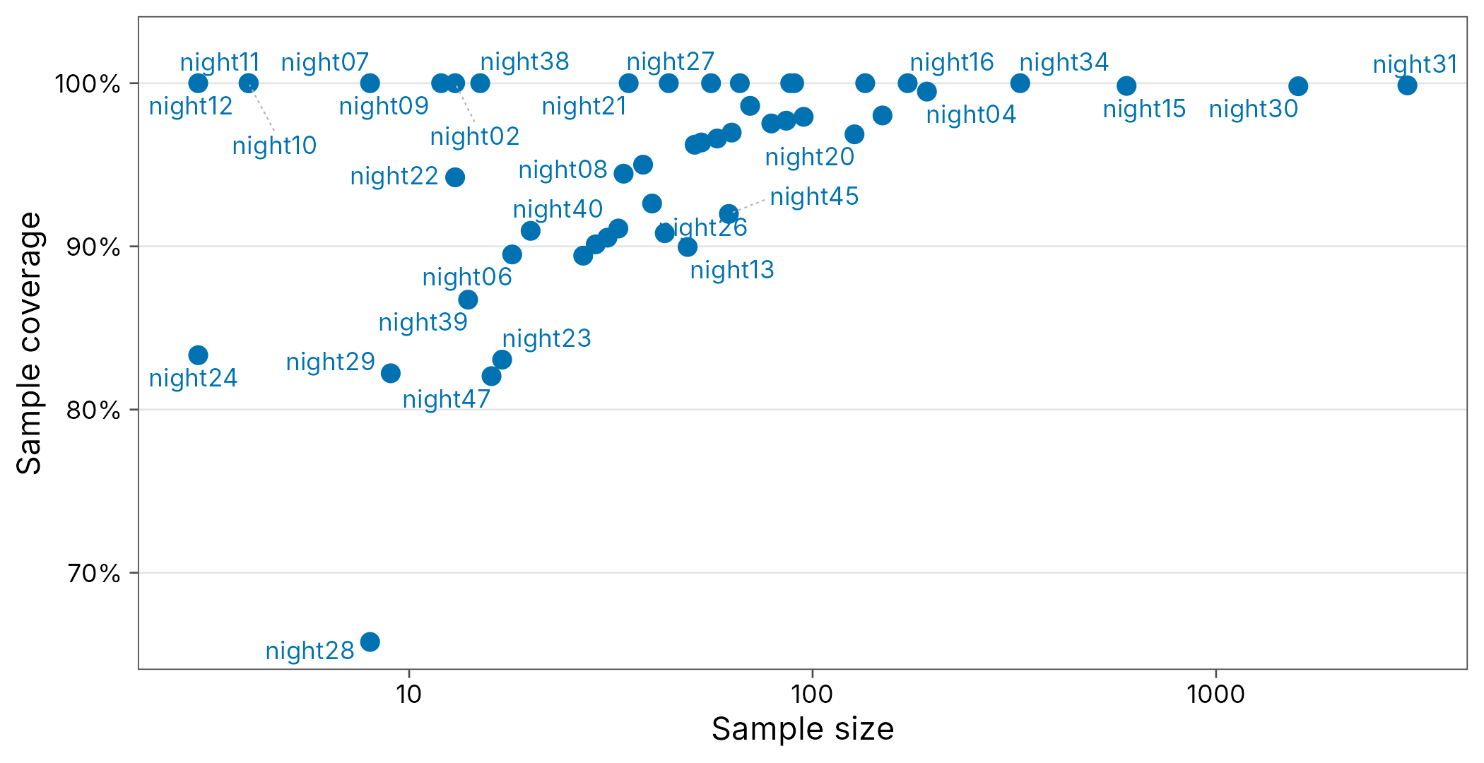

Desert rodents on the Portal Project exclosure experiment (bundled portal_rodents, CC0). Mixed models with plot as a random effect and multiple-site beta partitions. Full tutorial.

portal_rodents |>
  filter(year == 2019, treatment != "removal") |>
  mutate(site = treatment) |>
  div_rarefy(q = c(0, 1), nboot = 50) |>
  autoplot()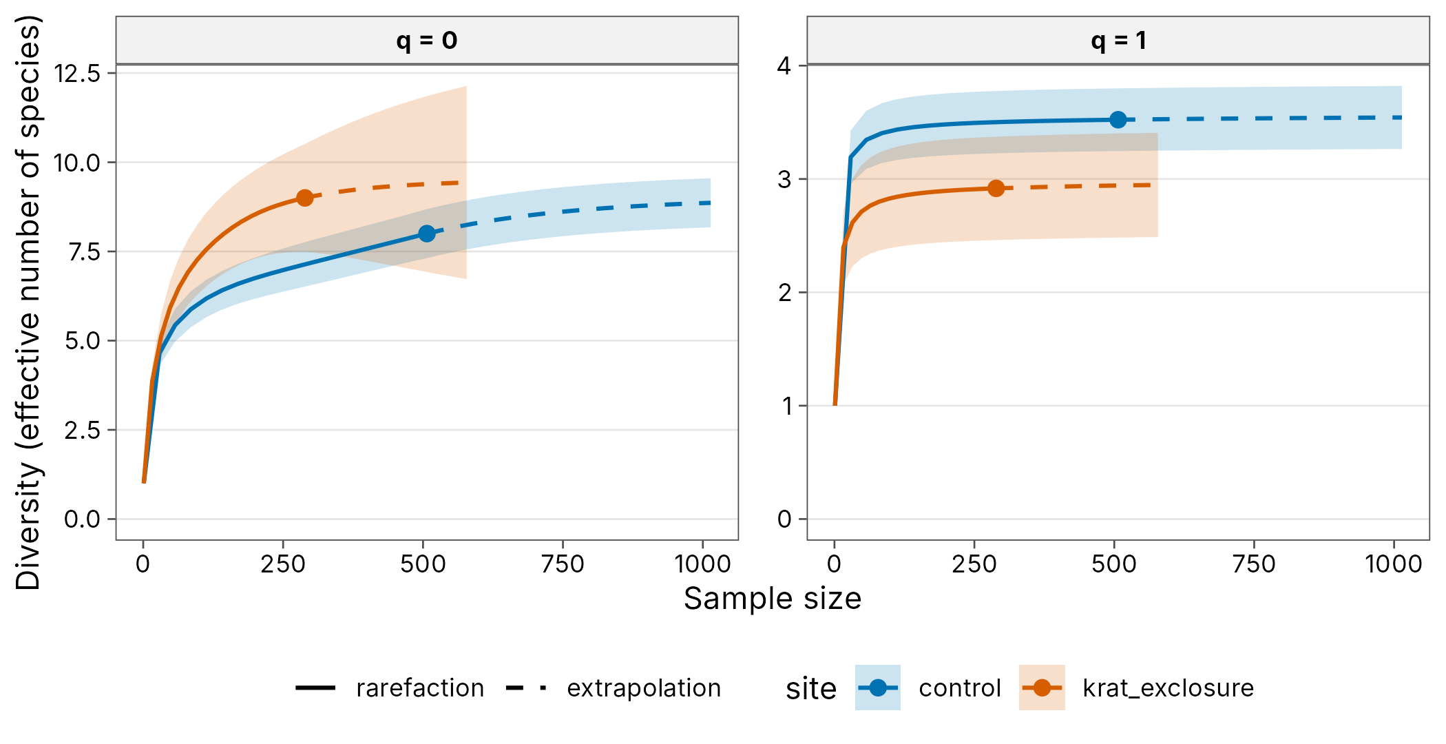

Forest birds in Taiwan (iNEXT bird) for alpha diversity, and the North American Breeding Bird Survey (betapart bbs1980, bbs2000) for spatial and temporal beta diversity. Full tutorial.

data(bird, package = "iNEXT")
birds <- tibble::tibble(
  species = seq_len(nrow(bird)),
  North = bird$North.site, South = bird$South.site
) |>
  tidyr::pivot_longer(-species,
    names_to = "site",
    values_to = "abundance"
  ) |>
  as_community()
autoplot(div_estimate(birds, nboot = 50))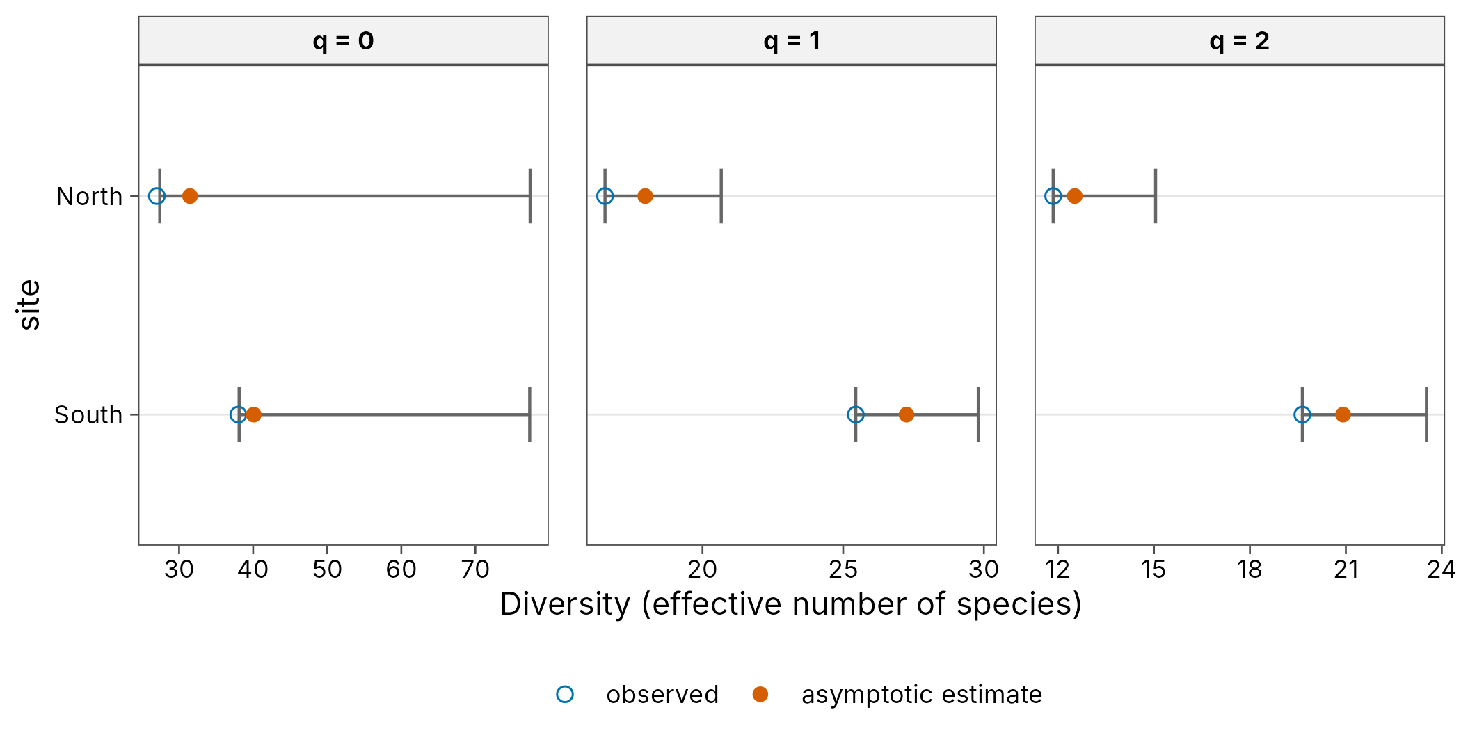

Trees in fifty 1 ha plots on Barro Colorado Island (vegan BCI), with habitat models, spatial distance decay, NMDS and PERMANOVA. Full tutorial.

data(BCI, package = "vegan")
trees <- community_long(bind_cols(site = c("ha01", "ha02"), BCI[1:2, ]),
  cols = -site
)
autoplot(div_hill(trees, q = seq(0, 3, by = 0.25)))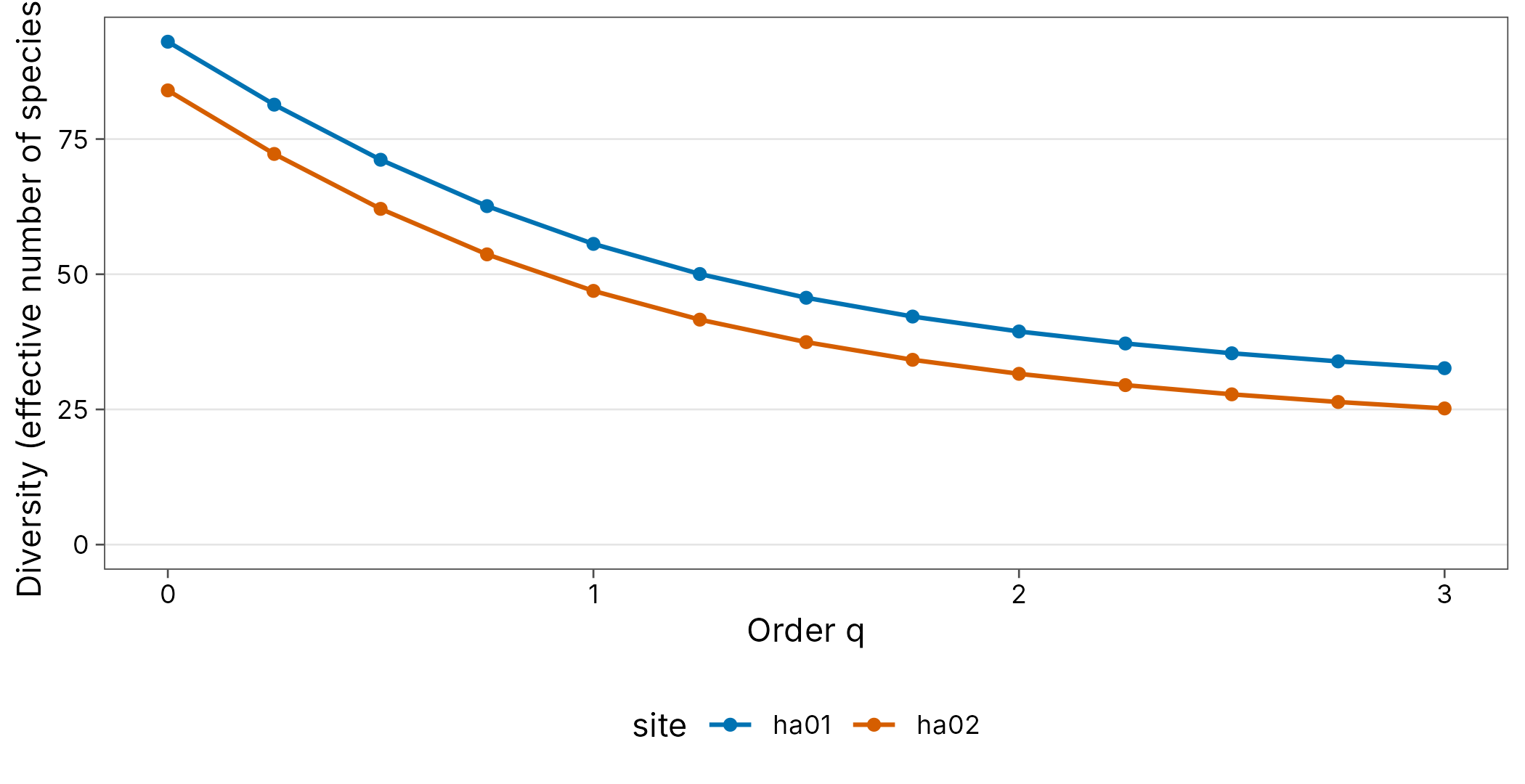

Which tutorial to start with

• PNG ants shows bait occurrence data, seasons and plots of individual trees.
• PNG frogs follows a near-complete inventory along a 3500 m elevational gradient.
• PNG butterflies shows temporal diversity from repeated monitoring of one plot.
• Insects shows coverage-based standardisation when sampling effort varies a lot between samples.
• Mammals shows mixed models with repeated surveys of the same plots.
• Birds compares assemblages directly against iNEXT and betapart reference data.
• Plants covers spatial beta diversity, PERMANOVA and ordination.

Data licences

The Papua New Guinea datasets come from Dryad and Zenodo deposits (png_tree_ants, png_frogs and wanang_butterflies under CC0 1.0; png_ants with the lead author’s permission). The other datasets come from CRAN packages (ade4, iNEXT, betapart, vegan) under GPL licences, or from the Portal Project (CC0). Each tutorial cites the original source.