Testing community composition • tidydiversity

Ordination shows patterns in composition. This article covers how to test them, following the standard workflow (Borcard, Gillet and Legendre 2018):

Does composition differ with site variables? (PERMANOVA)
Is that result caused by groups differing in spread? (dispersion test)
Which variables should enter the model? (forward selection)
How much does each group of variables explain on its own? (variation partitioning)
Which species characterise each group? (indicator species)

All results are tidy tibbles. The computations are done by vegan and indicspecies, and the test suite checks that the results are identical.

library(tidydiversity)
library(dplyr)
library(ggplot2)
set.seed(2026)

The units are the 20 transects of the Mt Wilhelm ant survey: 5 elevations x 2 seasons x 2 transects.

ants <- png_ants |>
  mutate(
    unit = paste(site, season, transect),
    zone = if_else(elevation <= 700, "lowland", "montane")
  )

1. PERMANOVA

beta_permanova(ants, site = unit, formula = ~ elevation + season)
#> # A tibble: 4 x 6
#>   term         df sum_sq     r2 statistic p.value
#>   <chr>     <dbl>  <dbl>  <dbl>     <dbl>   <dbl>
#> 1 elevation     1  1.33  0.169       3.75   0.001
#> 2 season        1  0.526 0.0669      1.49   0.101
#> 3 Residual     17  6.01  0.765      NA     NA    
#> 4 Total        19  7.87  1          NA     NA

Each term is tested after the other (by = "margin", the default), so the result does not depend on the order of terms in the formula. Here the design is balanced, so sequential tests (by = "terms", vegan’s default) give the same numbers; with correlated terms they would not.

Elevation explains 17% of the variation in composition (Bray-Curtis). To test season while respecting the paired design, permute only within sites:

beta_permanova(ants, site = unit, formula = ~season, strata = site)
#> # A tibble: 3 x 6
#>   term        df sum_sq     r2 statistic p.value
#>   <chr>    <dbl>  <dbl>  <dbl>     <dbl>   <dbl>
#> 1 season       1  0.526 0.0669      1.29   0.003
#> 2 Residual    18  7.34  0.933      NA     NA    
#> 3 Total       19  7.87  1          NA     NA

The season effect, hidden by the large differences between elevations, becomes clear once each transect is compared only with transects on its own site.

2. Homogeneity of dispersion

PERMANOVA can also give a significant result when groups differ in spread rather than in location (Anderson 2006). Check this:

disp <- beta_dispersion(ants, site = unit, group = season)
attr(disp, "test")
#> # A tibble: 2 x 5
#>   term         df  sum_sq statistic p.value
#>   <chr>     <int>   <dbl>     <dbl>   <dbl>
#> 1 Groups        1 0.00182     0.466   0.501
#> 2 Residuals    18 0.0702     NA      NA
autoplot(disp)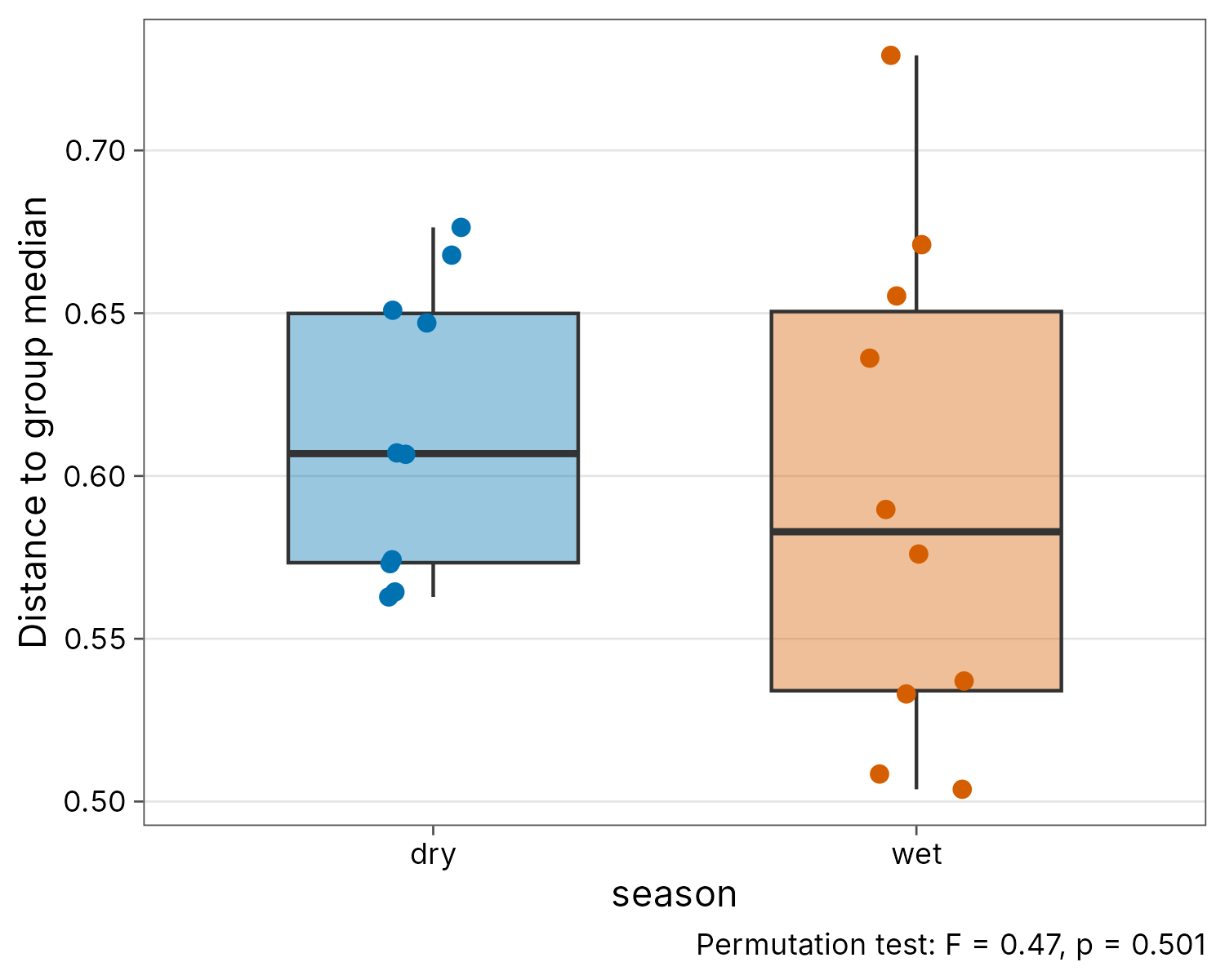

Boxplots of each transect's distance to its season's spatial median: dry and wet seasons overlap.

The seasons have similar dispersion, so a season effect is a real shift in composition, not a difference in spread.

When dispersions do differ, or group sizes are unbalanced, use the Welch-type PERMANOVA W*d (Hamidi et al. 2019), which stays valid under unequal spread:

set.seed(1)
beta_welch(ants, site = unit, group = season)
#> # A tibble: 1 x 4
#>   statistic n_groups n_sites p.value
#>       <dbl>    <int>   <int>   <dbl>
#> 1      1.29        2      20   0.179

3. Forward selection

With many candidate variables, select them by forward selection with the double stopping rule of Blanchet et al. (2008). It stops before the model explains more than the full model, to avoid inflated Type I error and an overfitted model:

sel <- ord_select(ants, site = unit, formula = ~ elevation + season)
sel
#> # A tibble: 1 x 5
#>    step term      adj_r2 statistic p.value
#>   <int> <chr>      <dbl>     <dbl>   <dbl>
#> 1     1 elevation  0.101      3.13   0.001
attr(sel, "adj_r2_full")
#> [1] 0.1135565

4. Variation partitioning

How much do elevation and season explain on their own and together (adjusted R², Peres-Neto et al. 2006)?

ord_varpart(ants, site = unit, elevation = ~elevation, season = ~season)
#> # A tibble: 4 x 5
#>   fraction        label                       adj_r2 testable p.value
#>   <chr>           <chr>                        <dbl> <lgl>      <dbl>
#> 1 [a] = X1|X2     elevation only             0.107   TRUE       0.001
#> 2 [b] = X2|X1     season only                0.0127  TRUE       0.171
#> 3 [c]             shared elevation & season -0.00631 FALSE     NA    
#> 4 [d] = Residuals residual                   0.886   FALSE     NA

Up to four groups of variables are allowed, for example climate, soil, space (from elevation or coordinates) and time.

5. Indicator species

Which species characterise lowland and montane transects (IndVal, De Caceres et al. 2010)? A is specificity, the probability that a site holding the species belongs to the group; B is fidelity, the proportion of the group’s sites holding the species. Because every species is tested, the p-values are corrected for multiple testing (Holm by default, column p.adj) before species are selected; use adjust = "fdr" for a less strict false discovery rate.

set.seed(1)
beta_indicator(ants, site = unit, group = zone)
#> # A tibble: 0 x 7
#> # i 7 variables: species <chr>, group <chr>, stat <dbl>, A <dbl>, B <dbl>,
#> #   p.value <dbl>, p.adj <dbl>

No species is a reliable indicator once the p-values are corrected. The uncorrected ranking shows why: of the 79 species tested, only a few reach p.value < 0.05, about as many as expected by chance alone.

set.seed(1)
beta_indicator(ants, site = unit, group = zone, adjust = "none", alpha = 1) |>
  dplyr::arrange(p.value) |>
  head()
#> # A tibble: 6 x 7
#>   species  group    stat     A     B p.value p.adj
#>   <chr>    <chr>   <dbl> <dbl> <dbl>   <dbl> <dbl>
#> 1 rhyt_001 lowland 0.707 1     0.5     0.014 0.014
#> 2 mono_002 lowland 0.761 0.927 0.625   0.016 0.016
#> 3 para_005 lowland 0.612 1     0.375   0.046 0.046
#> 4 oeco_001 lowland 0.612 1     0.375   0.053 0.053
#> 5 phei_003 lowland 0.612 1     0.375   0.055 0.055
#> 6 care_007 lowland 0.655 0.857 0.5     0.063 0.063

References

Anderson, M. J. (2001). A new method for non-parametric multivariate analysis of variance. Austral Ecology, 26, 32-46.

Anderson, M. J. (2006). Distance-based tests for homogeneity of multivariate dispersions. Biometrics, 62, 245-253.

Blanchet, F. G., Legendre, P. and Borcard, D. (2008). Forward selection of explanatory variables. Ecology, 89, 2623-2632.

Borcard, D., Gillet, F. and Legendre, P. (2018). Numerical Ecology with R, 2nd edn. Springer.

De Caceres, M., Legendre, P. and Moretti, M. (2010). Improving indicator species analysis by combining groups of sites. Oikos, 119, 1674-1684.

Hamidi, B. et al. (2019). Wd-test: robust distance-based multivariate analysis of variance. Microbiome*, 7, 51.

Legendre, P. and Legendre, L. (2012). Numerical Ecology, 3rd English edn. Elsevier.

Peres-Neto, P. R. et al. (2006). Variation partitioning of species data matrices: estimation and comparison of fractions. Ecology, 87, 2614-2625.