Case study: caddisflies at a light trap

This case study runs the full workflow on nightly light-trap catches of adult caddisflies (Trichoptera) from the Rhône, France. The data are the trichometeo dataset in the ade4 package: counts of 17 genera on 49 nights, with weather recorded on each night. Sampling effort differs greatly between nights, which makes it a good example of why diversity has to be standardised before it is compared.

Source and licence. Usseglio-Polatera, P. and Auda, Y. (1987). Influence des facteurs météorologiques sur les résultats de piégeage lumineux. Annales de Limnologie 23: 65-79. Distributed with ade4 (Dray and Dufour 2007; licence GPL-2 or later). The data are loaded from ade4 at run time and are not redistributed with tidydiversity.

library(tidydiversity)
library(dplyr)
library(ggplot2)
set.seed(2026)

Tidy the data

community_long() turns a site by species table into the long format used throughout the package. Covariate columns that are not selected stay with each record, and add_site_data() joins them back on later.

data(trichometeo, package = "ade4")
nights <- tibble::tibble(
  site = sprintf("night%02d", seq_len(nrow(trichometeo$fau))),
  evening_temp = trichometeo$meteo$T.soir,
  wind = trichometeo$meteo$Vent,
  humidity = trichometeo$meteo$Humidite,
  cloud = trichometeo$meteo$Nebu.Nuit
)
wide <- bind_cols(site = nights$site, trichometeo$fau)
moths <- community_long(wide, cols = -site)
moths
#> # A community: 49 sites, 17 species, 7,778 individuals
#>    site    species abundance
#>    <chr>   <chr>       <dbl>
#>  1 night01 All             1
#>  2 night01 Ced             2
#>  3 night01 Hfo             1
#>  4 night01 Hsp             2
#>  5 night01 Hym             5
#>  6 night01 Psy            17
#>  7 night01 Sta             1
#>  8 night02 All             2
#>  9 night02 Hym             3
#> 10 night02 Psy             8
#> # i 305 more rows

How complete is each night?

cov <- div_coverage(moths)
summary(cov$n)
#>    Min. 1st Qu.  Median    Mean 3rd Qu.    Max. 
#>     3.0    16.0    43.0   158.7    86.0  2980.0
autoplot(cov) + scale_x_log10()
#> Scale for x is already present.
#> Adding another scale for x, which will replace the existing scale.
#> Warning: ggrepel: 18 unlabeled data points (too many overlaps). Consider
#> increasing max.overlaps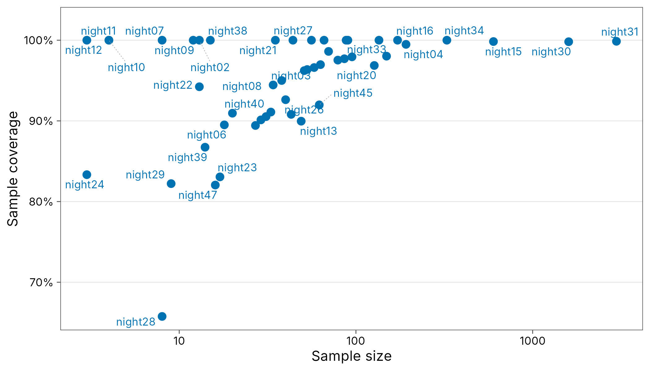

Catches range from a handful of insects to more than a thousand, so raw counts of genera mostly track trap effort. Sample coverage is high on most nights, so coverage-based standardisation is reliable here.

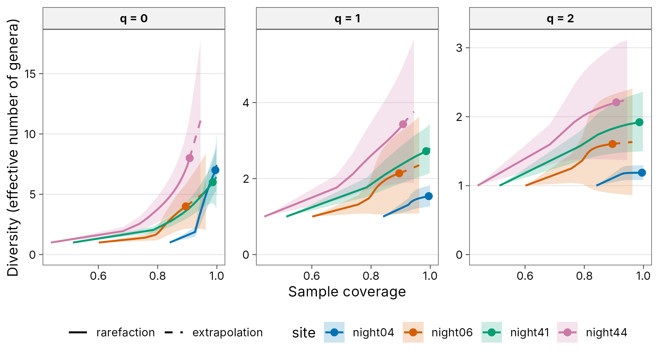
Rarefaction and extrapolation

A few contrasting nights show the shape of the curves. Plotting against sample coverage rather than the number of insects puts nights of very different size on a common scale. Solid lines are interpolated, dashed lines extrapolated, and ribbons are 95% bootstrap intervals.

pick <- cov |>
  arrange(n) |>
  slice(c(15, 25, 35, 45)) |>
  pull(site)
curves <- div_rarefy(filter(moths, site %in% pick), nboot = 100)
autoplot(curves,
  x = "coverage", ncol = 3,
  ylab = "Diversity (effective number of genera)"
)

Standardised diversity for every night

Nights with too few insects to estimate anything are dropped first.

keep <- cov |>
  filter(n >= 20, s_obs >= 2) |>
  pull(site)
std <- div_standardise(filter(moths, site %in% keep),
  q = c(0, 1, 2),
  nboot = 100
)
distinct(std, coverage)
#> # A tibble: 34 x 1
#>    coverage
#>       <dbl>
#>  1    0.945
#>  2    0.945
#>  3    0.945
#>  4    0.945
#>  5    0.945
#>  6    0.945
#>  7    0.945
#>  8    0.945
#>  9    0.945
#> 10    0.945
#> # i 24 more rows
std
#> # A tibble: 102 x 9
#>    site        q     m method        coverage diversity     se lower upper
#>    <chr>   <dbl> <dbl> <chr>            <dbl>     <dbl>  <dbl> <dbl> <dbl>
#>  1 night01     0  41.5 extrapolation    0.945      7.96 1.57    4.87 11.0 
#>  2 night01     1  41.5 extrapolation    0.945      4.02 0.817   2.42  5.62
#>  3 night01     2  41.5 extrapolation    0.945      2.63 0.555   1.54  3.72
#>  4 night03     0  25.5 rarefaction      0.945      3.33 0.457   2.44  4.23
#>  5 night03     1  25.5 rarefaction      0.945      1.72 0.254   1.23  2.22
#>  6 night03     2  25.5 rarefaction      0.945      1.38 0.178   1.03  1.73
#>  7 night04     0  36.5 rarefaction      0.945      3.52 0.412   2.71  4.33
#>  8 night04     1  36.5 rarefaction      0.945      1.43 0.105   1.23  1.64
#>  9 night04     2  36.5 rarefaction      0.945      1.18 0.0469  1.09  1.28
#> 10 night05     0  40.3 rarefaction      0.945      4.49 0.681   3.16  5.83
#> # i 92 more rows

Diversity and weather

tidy() gives model-ready columns, including an inverse-variance weight, and add_site_data() brings the weather covariates in.

shannon <- std |>
  tidy() |>
  filter(q == 1) |>
  add_site_data(nights)

fit <- lm(estimate ~ evening_temp + wind + humidity,
  data = shannon,
  weights = weight
)
broom::tidy(fit, conf.int = TRUE)
#> # A tibble: 4 x 7
#>   term         estimate std.error statistic p.value conf.low conf.high
#>   <chr>           <dbl>     <dbl>     <dbl>   <dbl>    <dbl>     <dbl>
#> 1 (Intercept)    5.87      3.34       1.76   0.0894  -0.959    12.7   
#> 2 evening_temp  -0.116     0.0773    -1.50   0.144   -0.274     0.0418
#> 3 wind          -0.0540    0.0600    -0.901  0.375   -0.177     0.0685
#> 4 humidity      -0.0140    0.0241    -0.580  0.566   -0.0631    0.0352

ggplot(shannon, aes(evening_temp, estimate)) +
  geom_pointrange(aes(ymin = conf.low, ymax = conf.high),
    colour = plot_palette(1)
  ) +
  geom_smooth(
    method = "lm", formula = y ~ x,
    mapping = aes(weight = weight), colour = "grey30"
  ) +
  labs(
    x = "Evening air temperature (\u00b0C)",
    y = "Shannon diversity (effective number of genera)"
  ) +
  theme_tidydiversity()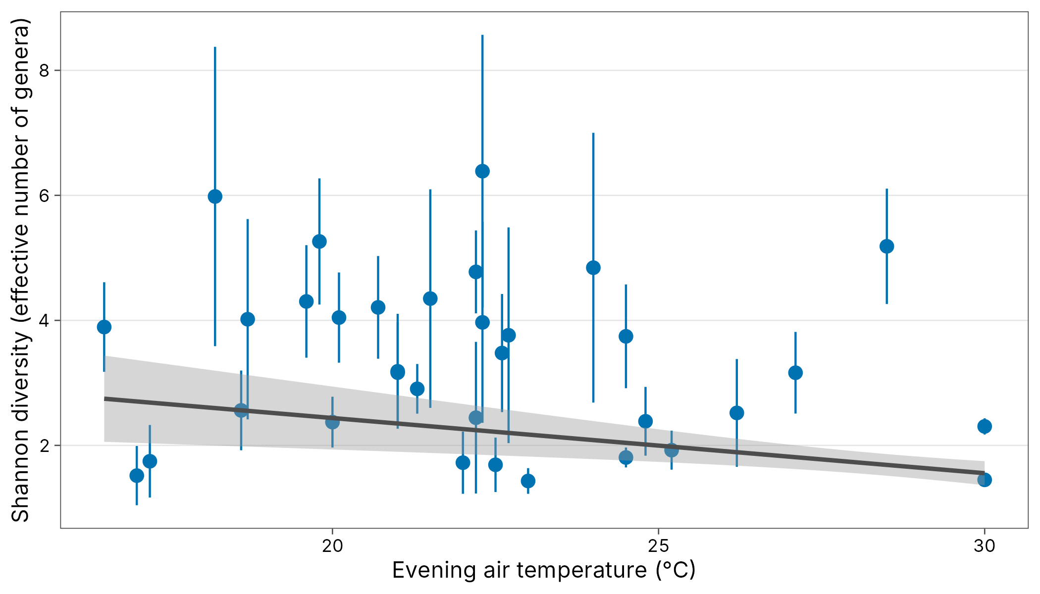

Beta diversity between nights

Abundance-based Bray-Curtis dissimilarity, split into balanced variation (turnover) and abundance gradients (nestedness), against the difference in evening temperature.

decay <- moths |>
  filter(site %in% keep) |>
  left_join(nights, by = "site") |>
  beta_decay(gradient = evening_temp, index = "bray")
autoplot(decay, xlab = "Difference in evening temperature (\u00b0C)")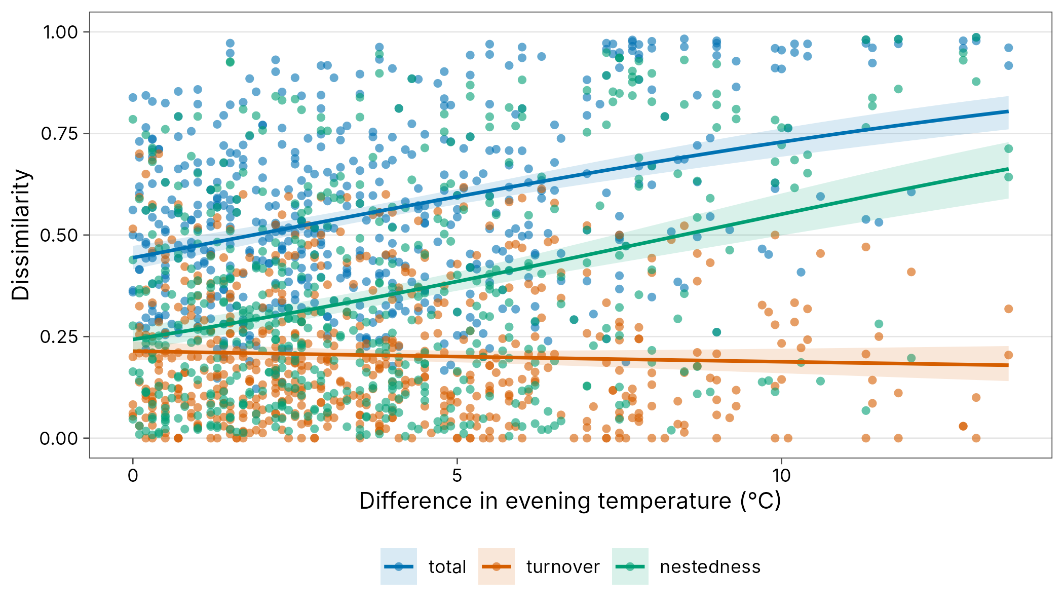

Reporting

div_table(filter(std, site %in% keep[1:6]),
  digits = 1, wide = TRUE,
  output = "kable", caption = "Coverage-standardised diversity, first six nights"
)

Coverage-standardised diversity, first six nights

site	q = 0	q = 1	q = 2
night01	8.0 [4.9, 11.0]	4.0 [2.4, 5.6]	2.6 [1.5, 3.7]
night03	3.3 [2.4, 4.2]	1.7 [1.2, 2.2]	1.4 [1.0, 1.7]
night04	3.5 [2.7, 4.3]	1.4 [1.2, 1.6]	1.2 [1.1, 1.3]
night05	4.5 [3.2, 5.8]	1.7 [1.3, 2.1]	1.3 [1.1, 1.5]
night08	4.0 [2.7, 5.3]	1.7 [1.2, 2.3]	1.4 [1.0, 1.7]
night13	10.8 [5.6, 15.9]	2.4 [1.2, 3.7]	1.5 [1.0, 2.0]

References

Chao, A., Gotelli, N. J., Hsieh, T. C., et al. (2014). Rarefaction and extrapolation with Hill numbers. Ecological Monographs 84: 45-67.

Dray, S. and Dufour, A.-B. (2007). The ade4 package. Journal of Statistical Software 22(4): 1-20.