library(tidydiversity)
library(dplyr)
#>
#> Attaching package: 'dplyr'
#> The following objects are masked from 'package:stats':
#>
#>     filter, lag
#> The following objects are masked from 'package:base':
#>
#>     intersect, setdiff, setequal, union
library(ggplot2)
set.seed(42)
The examples use png_ants: ants recorded at nutrient
baits along the Mt Wilhelm elevational gradient in Papua New Guinea, in
the dry and wet seasons (Moses et al. 2023). Each bait at which a
species was found counts as one occurrence.
Hill numbers
Hill numbers express diversity as an effective number of species.
Order q = 0 is richness, q = 1 weights species
by their frequency and q = 2 emphasises the dominant
species.
div_hill(png_ants, q = c(0, 1, 2), .by = season)
#> # A tibble: 30 x 5
#>    season site       q     n diversity
#>    <chr>  <chr>  <dbl> <dbl>     <dbl>
#>  1 dry    MW0200     0    47     16
#>  2 dry    MW0200     1    47     12.3
#>  3 dry    MW0200     2    47      9.91
#>  4 wet    MW0200     0    76     21
#>  5 wet    MW0200     1    76     10.9
#>  6 wet    MW0200     2    76      6.99
#>  7 dry    MW0700     0    23     15
#>  8 dry    MW0700     1    23     11.8
#>  9 dry    MW0700     2    23      8.67
#> 10 wet    MW0700     0    58     28
#> # i 20 more rows
Sample coverage
Raw counts depend on sampling effort. Sample coverage estimates how complete each sample is.
div_coverage(png_ants, .by = season)
#> # A tibble: 10 x 7
#>    season site       n s_obs    f1    f2 coverage
#>    <chr>  <chr>  <dbl> <int> <int> <int>    <dbl>
#>  1 dry    MW0200    47    16     5     5    0.898
#>  2 wet    MW0200    76    21    11     5    0.857
#>  3 dry    MW0700    23    15    12     1    0.482
#>  4 wet    MW0700    58    28    17     3    0.709
#>  5 dry    MW1200    29    13     7     3    0.766
#>  6 wet    MW1200    57    20     9     3    0.844
#>  7 dry    MW1700    17     5     1     2    0.953
#>  8 wet    MW1700    34    10     6     2    0.827
#>  9 dry    MW2200    13     6     3     1    0.781
#> 10 wet    MW2200    15     5     2     1    0.876
Asymptotic estimates
div_estimate() gives Chao1 richness, the Chao et
al. (2013) Shannon estimator and the unbiased Simpson estimator, with
bootstrap intervals.
div_estimate(png_ants, .by = season, nboot = 50) |>
  filter(q == 0)
#> # A tibble: 10 x 8
#>    season site       q observed estimate    se lower upper
#>    <chr>  <chr>  <dbl>    <dbl>    <dbl> <dbl> <dbl> <dbl>
#>  1 dry    MW0200     0       16    18.4   3.55 16.3   35.7
#>  2 wet    MW0200     0       21    32.9  12.5  23.2   85.3
#>  3 dry    MW0700     0       15    83.9  31.2  44.5  176.
#>  4 wet    MW0700     0       28    75.3  54.2  35.9  313.
#>  5 dry    MW1200     0       13    20.9   9.83 14.2   65.6
#>  6 wet    MW1200     0       20    33.3  15.3  22.2  101.
#>  7 dry    MW1700     0        5     5.24  2.11  5.00  19.4
#>  8 wet    MW1700     0       10    18.7   8.09 11.9   50.8
#>  9 dry    MW2200     0        6    10.2   4.35  6.77  28.5
#> 10 wet    MW2200     0        5     6.87  2.30  5.28  17.3
Rarefaction and extrapolation
div_rarefy() interpolates each sample down to smaller
sizes and extrapolates up to twice its size. The values match the iNEXT
package.
curves <- png_ants |>
  filter(season == "wet") |>
  div_rarefy(q = c(0, 1, 2), nboot = 30)
curves
#> # A tibble: 570 x 8
#>    site       q     m method      diversity coverage lower upper
#>    <chr>  <dbl> <dbl> <chr>           <dbl>    <dbl> <dbl> <dbl>
#>  1 MW0200     0     1 rarefaction      1       0.132  1     1.00
#>  2 MW0200     0     5 rarefaction      3.92    0.445  3.54  4.30
#>  3 MW0200     0     9 rarefaction      5.90    0.585  5.07  6.73
#>  4 MW0200     0    13 rarefaction      7.44    0.655  6.21  8.67
#>  5 MW0200     0    17 rarefaction      8.75    0.695  7.16 10.3
#>  6 MW0200     0    21 rarefaction      9.93    0.721  8.00 11.9
#>  7 MW0200     0    25 rarefaction     11.0     0.740  8.78 13.3
#>  8 MW0200     0    29 rarefaction     12.0     0.754  9.51 14.6
#>  9 MW0200     0    33 rarefaction     13.0     0.766 10.2  15.8
#> 10 MW0200     0    38 rarefaction     14.1     0.780 11.0  17.3
#> # i 560 more rows
autoplot(curves)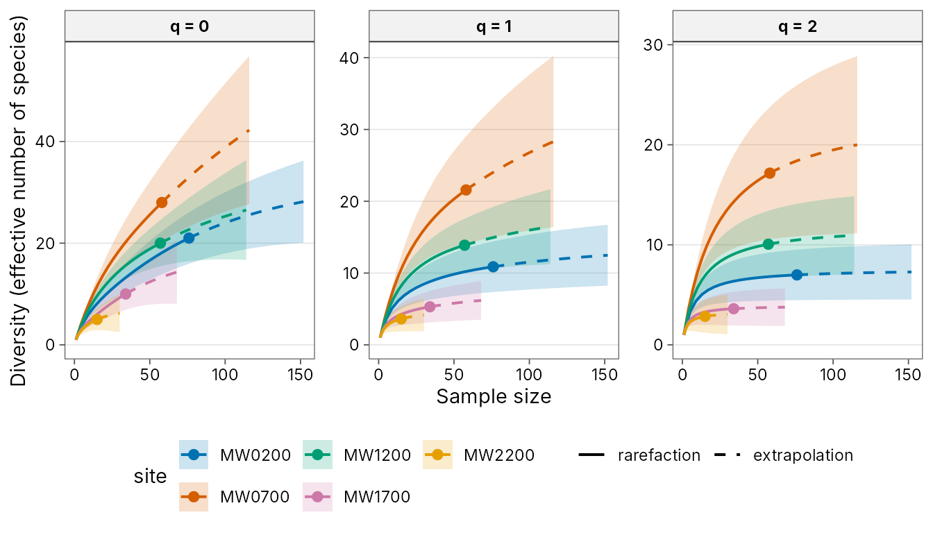
Plotting against coverage shows how complete each sample is:
autoplot(curves, x = "coverage")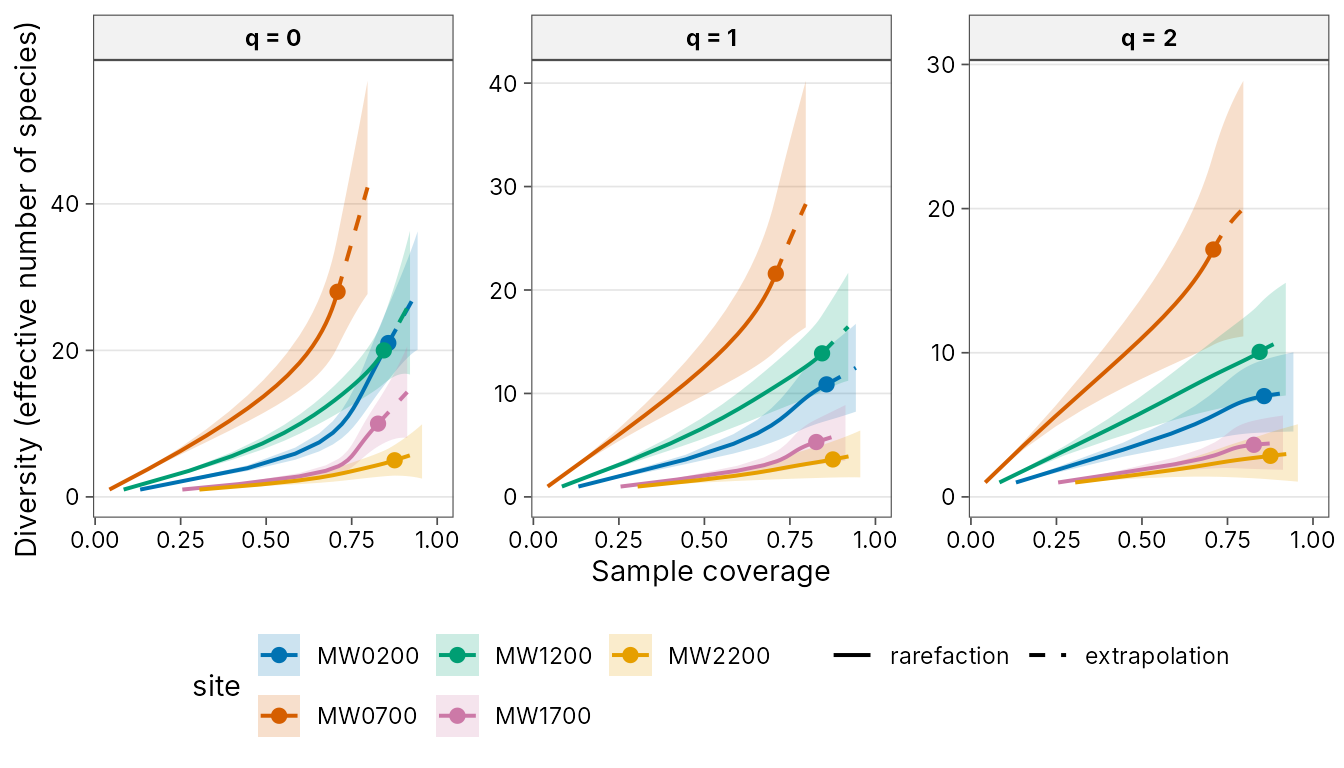
Fair comparisons
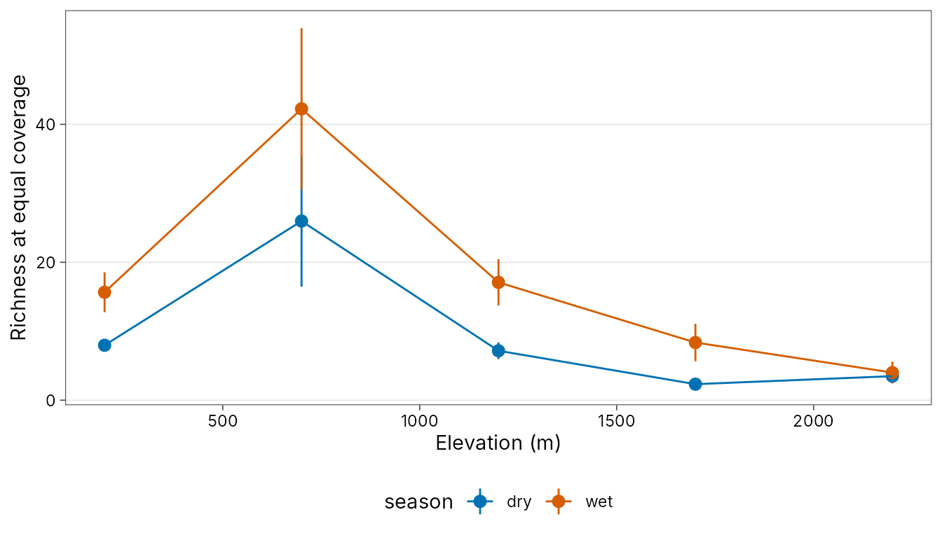
Compare sites at equal completeness with
div_standardise(). With no level given, each group is
standardised to the lowest coverage that its sites reach at twice their
sample size.
std <- div_standardise(png_ants, .by = season, nboot = 50)
std
#> # A tibble: 30 x 10
#>    season site       q     m method        coverage diversity    se  lower upper
#>    <chr>  <chr>  <dbl> <dbl> <chr>            <dbl>     <dbl> <dbl>  <dbl> <dbl>
#>  1 dry    MW0200     0  11.6 rarefaction      0.565      7.96 0.444  7.09   8.83
#>  2 dry    MW0200     1  11.6 rarefaction      0.565      7.10 0.502  6.11   8.08
#>  3 dry    MW0200     2  11.6 rarefaction      0.565      6.24 0.526  5.21   7.27
#>  4 wet    MW0200     0  45.1 rarefaction      0.796     15.7  1.47  12.8   18.5
#>  5 wet    MW0200     1  45.1 rarefaction      0.796      9.57 1.24   7.14  12.0
#>  6 wet    MW0200     2  45.1 rarefaction      0.796      6.63 0.914  4.84   8.42
#>  7 dry    MW0700     0  46.0 extrapolation    0.565     26.0  4.86  16.5   35.5
#>  8 dry    MW0700     1  46.0 extrapolation    0.565     17.9  5.71   6.67  29.0
#>  9 dry    MW0700     2  46.0 extrapolation    0.565     10.5  5.07   0.566 20.4
#> 10 wet    MW0700     0 116   extrapolation    0.796     42.2  5.97  30.5   53.9
#> # i 20 more rows
std |>
  left_join(distinct(png_ants, site, elevation), by = "site") |>
  filter(q == 0) |>
  ggplot(aes(elevation, diversity, colour = season)) +
  geom_pointrange(aes(ymin = lower, ymax = upper)) +
  geom_line() +
  labs(x = "Elevation (m)", y = "Richness at equal coverage") +
  scale_colour_tidydiversity() +
  theme_tidydiversity()