Ordination: biplots and triplots

ord_fit() fits every common ordination to long community data and returns tidy scores; autoplot() draws publication-quality biplots and triplots in the style of CANOCO. The ordinations are computed by the vegan package, so the results are identical to vegan’s (this is checked in the test suite).

library(tidydiversity)
library(dplyr)
library(ggplot2)
set.seed(2026)

Choosing a method

Question	Method	method =
Main gradients in composition, short gradients	Principal components analysis	"pca"
Main gradients, long gradients (species turn over)	Correspondence analysis, detrended CA	"ca", "dca"
Main gradients from any dissimilarity	Principal coordinates analysis, NMDS	"pcoa", "nmds"
How much composition do my variables explain?	Redundancy analysis	"rda"
The same, for long gradients	Canonical correspondence analysis	"cca"
The same, for any dissimilarity	Distance-based RDA	"dbrda"

A first DCA axis longer than about 4 standard deviation units suggests long gradients, where the unimodal methods (CA, CCA) fit better than the linear ones (PCA, RDA). PCA and RDA use the Hellinger transformation by default (Legendre and Gallagher 2001); change it with transform.

Reading the diagrams

Element	Meaning
Points	Sites (coloured by a site variable)
Red arrows from the origin	Species, in linear methods (PCA, RDA, PCoA, db-RDA): the direction in which each species increases
Red crosses	Species optima, in unimodal methods (CA, CCA, DCA) and NMDS
Dark arrows from the origin	Quantitative environmental variables; in NMDS and PCA they are fitted afterwards (passive)
Dark triangles	Centroids of factor levels, such as years
Ellipses, hulls, spiders	Spread of each group of sites
Faint dotted grey lines	Label leaders only: they join a label that was moved to avoid overlap to its point

Constrained ordination: butterflies at Wanang

wanang_butterflies holds butterfly counts on 36 days over three years. Does the community differ between years and change through the months? Site variables (here year and month) are taken from the data automatically, because they are constant within each day.

butterflies <- mutate(wanang_butterflies, year = factor(paste("Year", year)))
rda <- ord_fit(butterflies, method = "rda", formula = ~ year + month)
rda
#> RDA of 36 sites and 189 species
#> Transformation: hellinger
#> Variation explained: RDA1 13.1%, RDA2 6.4%, RDA3 4.1%
#> Constrained: 23.6% of the total

Permutation tests of the whole model and of each term:

ord_test(rda)
#> # A tibble: 2 x 5
#>   term        df variance statistic p.value
#>   <chr>    <dbl>    <dbl>     <dbl>   <dbl>
#> 1 Model        3   0.0521      3.29   0.001
#> 2 Residual    32   0.169      NA     NA
ord_test(rda, by = "terms")
#> # A tibble: 3 x 5
#>   term        df variance statistic p.value
#>   <chr>    <dbl>    <dbl>     <dbl>   <dbl>
#> 1 year         2   0.0336      3.18   0.001
#> 2 month        1   0.0185      3.51   0.001
#> 3 Residual    32   0.169      NA     NA

A triplot shows the days (points), the species with the strongest responses (red arrows), the month gradient (blue arrow) and the year centroids (triangles). Ellipses cover one standard deviation of the days in each year.

autoplot(rda, colour = year, ellipse = "sd", species = 10)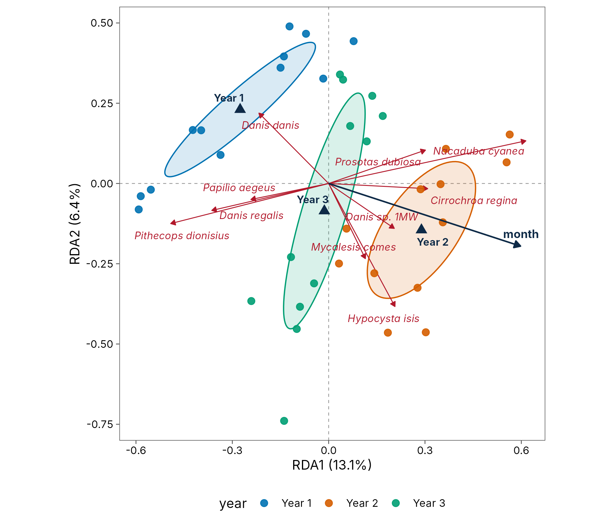

Unconstrained ordination with passive variables

NMDS summarises composition without reference to the variables; adding a formula fits them passively afterwards ([vegan::envfit()]), as supplementary variables in CANOCO.

nmds <- ord_fit(butterflies, method = "nmds", formula = ~ month + year)
tidy(nmds, "envfit")
#> # A tibble: 2 x 4
#>   term  type      r2 p.value
#>   <chr> <chr>  <dbl>   <dbl>
#> 1 month vector 0.198   0.034
#> 2 year  factor 0.185   0.01

autoplot(nmds, colour = month, group = year, hull = TRUE, species = 8)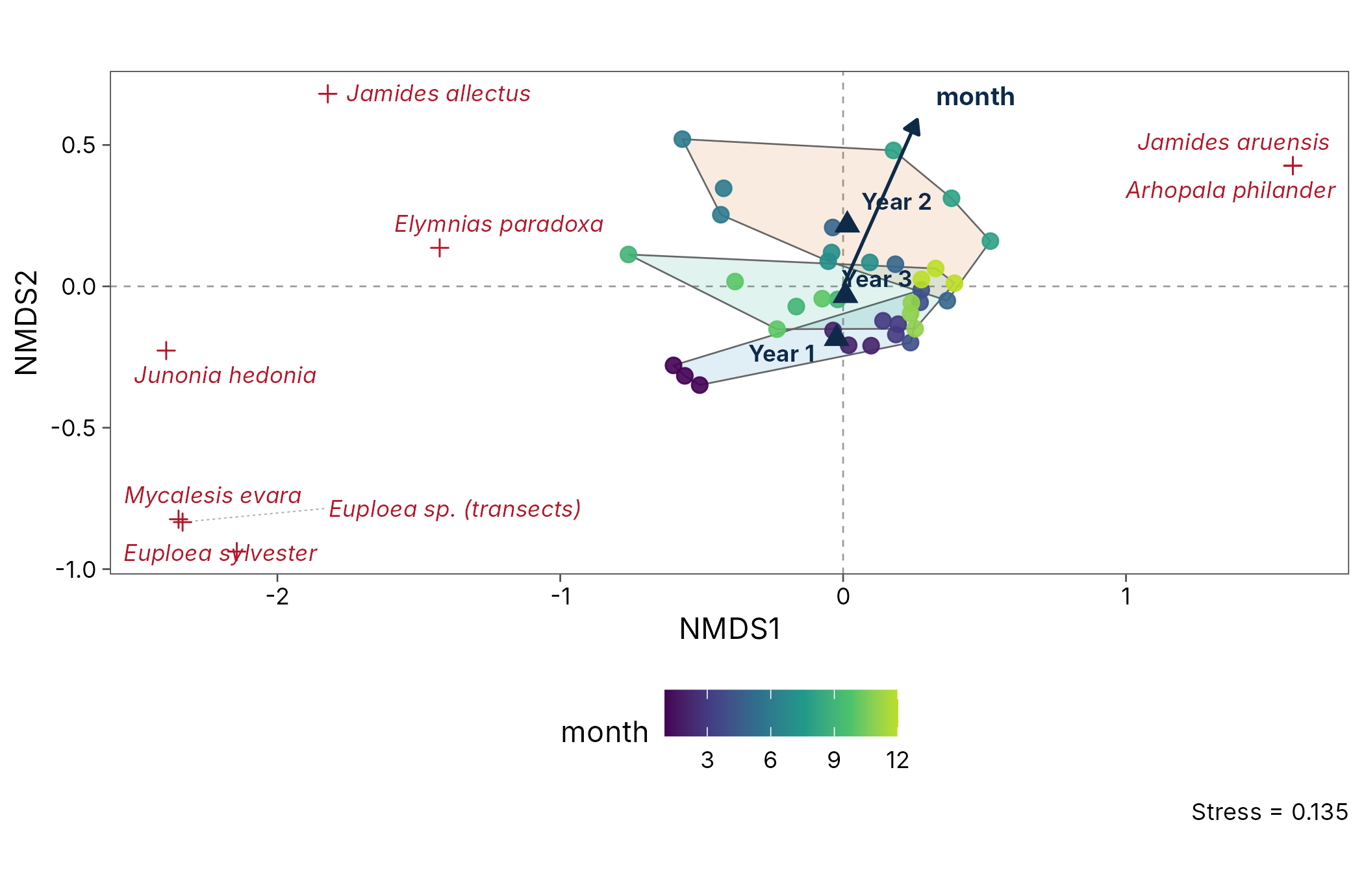

Frogs along Mt Wilhelm

Frog communities turn over almost completely along the elevational gradient, so a unimodal method suits them. CCA constrained by elevation:

cca <- ord_fit(png_frogs, method = "cca", formula = ~elevation)
ord_test(cca)
#> # A tibble: 2 x 5
#>   term        df chi_square statistic p.value
#>   <chr>    <dbl>      <dbl>     <dbl>   <dbl>
#> 1 Model        1      0.959      1.44   0.001
#> 2 Residual     6      4.00      NA     NA

autoplot(cca, colour = elevation, site_labels = TRUE, species = 12)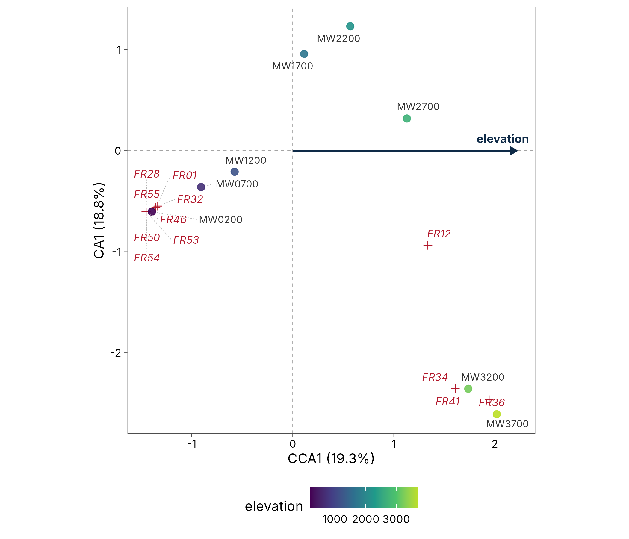

Customising the plot

Every option is an argument, and the result is an ordinary ggplot:

• axes = c(1, 3) plots other axes.
• species sets how many species to show (the best represented); 0 hides them.
• ellipse = "sd", "ci" (a level region for the points) or "se" (a level confidence region for the centroid); hull = TRUE; spider = TRUE.
• site_labels = TRUE, arrows = FALSE.
• colour, shape and group take site variables.

autoplot(rda, colour = year, shape = year, spider = TRUE, species = 0) +
  labs(title = "Butterfly communities at Wanang, by year") +
  theme(legend.position = "right")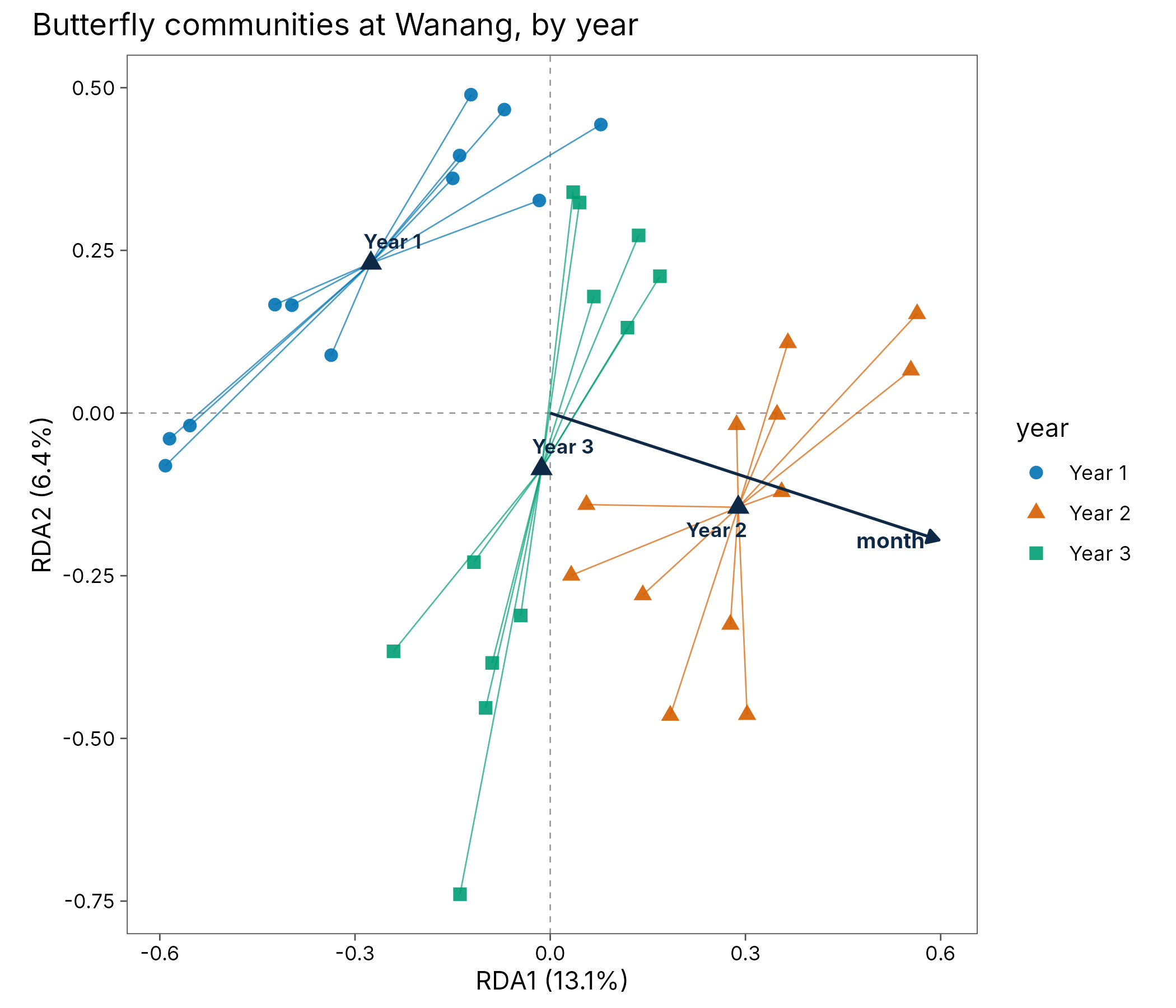

Tidy scores for your own plots

tidy(rda, "sites")
#> # A tibble: 36 x 7
#>    site    axis1   axis2    axis3   day month year  
#>    <chr>   <dbl>   <dbl>    <dbl> <int> <int> <fct> 
#>  1 day01 -0.554  -0.0192 -0.548       1     1 Year 1
#>  2 day02 -0.585  -0.0395 -0.437       2     1 Year 1
#>  3 day03 -0.591  -0.0809 -0.531       3     1 Year 1
#>  4 day04 -0.423   0.167  -0.0389      4     2 Year 1
#>  5 day05 -0.337   0.0890 -0.00424     5     2 Year 1
#>  6 day06 -0.397   0.166   0.119       6     2 Year 1
#>  7 day07 -0.0705  0.466  -0.0135      7     3 Year 1
#>  8 day08 -0.139   0.396  -0.0547      8     3 Year 1
#>  9 day09 -0.150   0.361  -0.0338      9     3 Year 1
#> 10 day10  0.0778  0.443  -0.191      10     4 Year 1
#> # i 26 more rows
tidy(rda, "axes")
#> # A tibble: 3 x 4
#>   axis  name  eigenvalue explained
#>   <chr> <chr>      <dbl>     <dbl>
#> 1 axis1 RDA1     0.0290     0.131 
#> 2 axis2 RDA2     0.0141     0.0637
#> 3 axis3 RDA3     0.00903    0.0409
glance(rda)
#> # A tibble: 1 x 8
#>   method n_sites n_species transform distance scaling stress constrained
#>   <chr>    <int>     <int> <chr>     <lgl>    <chr>    <dbl>       <dbl>
#> 1 rda         36       189 hellinger NA       species     NA       0.236

References

Legendre, P. and Gallagher, E. D. (2001). Ecologically meaningful transformations for ordination of species data. Oecologia, 129, 271-280. https://doi.org/10.1007/s004420100716

ter Braak, C. J. F. and Smilauer, P. (2012). Canoco reference manual and user’s guide: software for ordination (version 5.0). Microcomputer Power, Ithaca, USA.

Oksanen, J. et al. vegan: Community Ecology Package. https://CRAN.R-project.org/package=vegan