
Case study: desert rodents under experimental exclosures
Source:vignettes/articles/case-mammals.Rmd
case-mammals.RmdThe Portal Project is a long-term experiment in the Chihuahuan
Desert, Arizona, where rodents have been live-trapped on 24 fenced plots
since 1977. Some plots are open to all rodents (controls), some exclude
kangaroo rats (Dipodomys) through small gates, and some exclude
every rodent. The bundled portal_rodents dataset holds
counts of identified rodents on each plot in each year from 2016 to
2019.
Source and licence. PortalData, released under CC0
1.0. Cite as Ernest et al. (2020), below. See
?portal_rodents and data-raw/portal_rodents.R
for how it was built.
library(tidydiversity)
library(dplyr)
library(ggplot2)
set.seed(2026)
portal_rodents
#> # A tibble: 491 x 7
#>    site      plot  year treatment species scientific_name           abundance
#>    <chr>    <int> <int> <fct>     <chr>   <chr>                         <int>
#>  1 P01-2016     1  2016 removal   PM      Peromyscus maniculatus            9
#>  2 P01-2016     1  2016 removal   PE      Peromyscus eremicus               8
#>  3 P01-2016     1  2016 removal   RM      Reithrodontomys megalotis         6
#>  4 P01-2016     1  2016 removal   PP      Chaetodipus penicillatus          5
#>  5 P01-2016     1  2016 removal   PL      Peromyscus leucopus               1
#>  6 P01-2017     1  2017 removal   PP      Chaetodipus penicillatus         16
#>  7 P01-2017     1  2017 removal   OT      Onychomys torridus                9
#>  8 P01-2017     1  2017 removal   PL      Peromyscus leucopus               8
#>  9 P01-2017     1  2017 removal   PE      Peromyscus eremicus               6
#> 10 P01-2017     1  2017 removal   RM      Reithrodontomys megalotis         5
#> # i 481 more rows
count(distinct(portal_rodents, site, treatment), treatment)
#> # A tibble: 3 x 2
#>   treatment          n
#>   <fct>          <int>
#> 1 control           40
#> 2 krat_exclosure    32
#> 3 removal           24
The removal plots catch very few animals by design, so diversity is compared between control and kangaroo rat exclosure plots.
rodents <- filter(portal_rodents, treatment != "removal")
plots <- distinct(rodents, site, plot, year, treatment)
Sampling completeness
cov <- div_coverage(rodents)
autoplot(cov)
#> Warning: ggrepel: 30 unlabeled data points (too many overlaps). Consider
#> increasing max.overlaps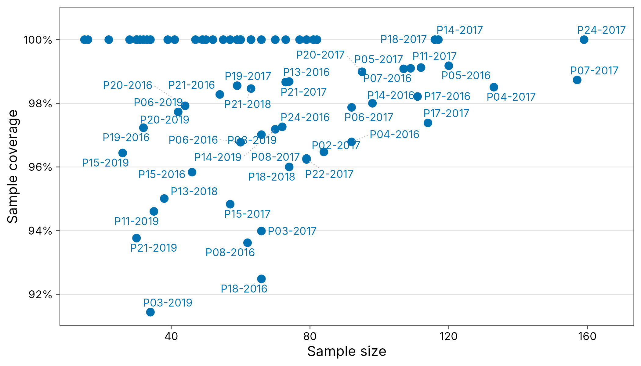
range(cov$coverage)
#> [1] 0.9143599 1.0000000
Coverage is above 90% almost everywhere, so differences in trapping success matter far less than they would for raw species counts.
Curves for each treatment
Pooling plots within each treatment and year gives one curve per
treatment, with 95% bootstrap ribbons. Results computed with
.by are faceted by group automatically.
pooled <- rodents |>
  mutate(site = treatment) |>
  as_community(.by = year)
curves <- div_rarefy(pooled, q = c(0, 1), .by = year, nboot = 100)
autoplot(curves)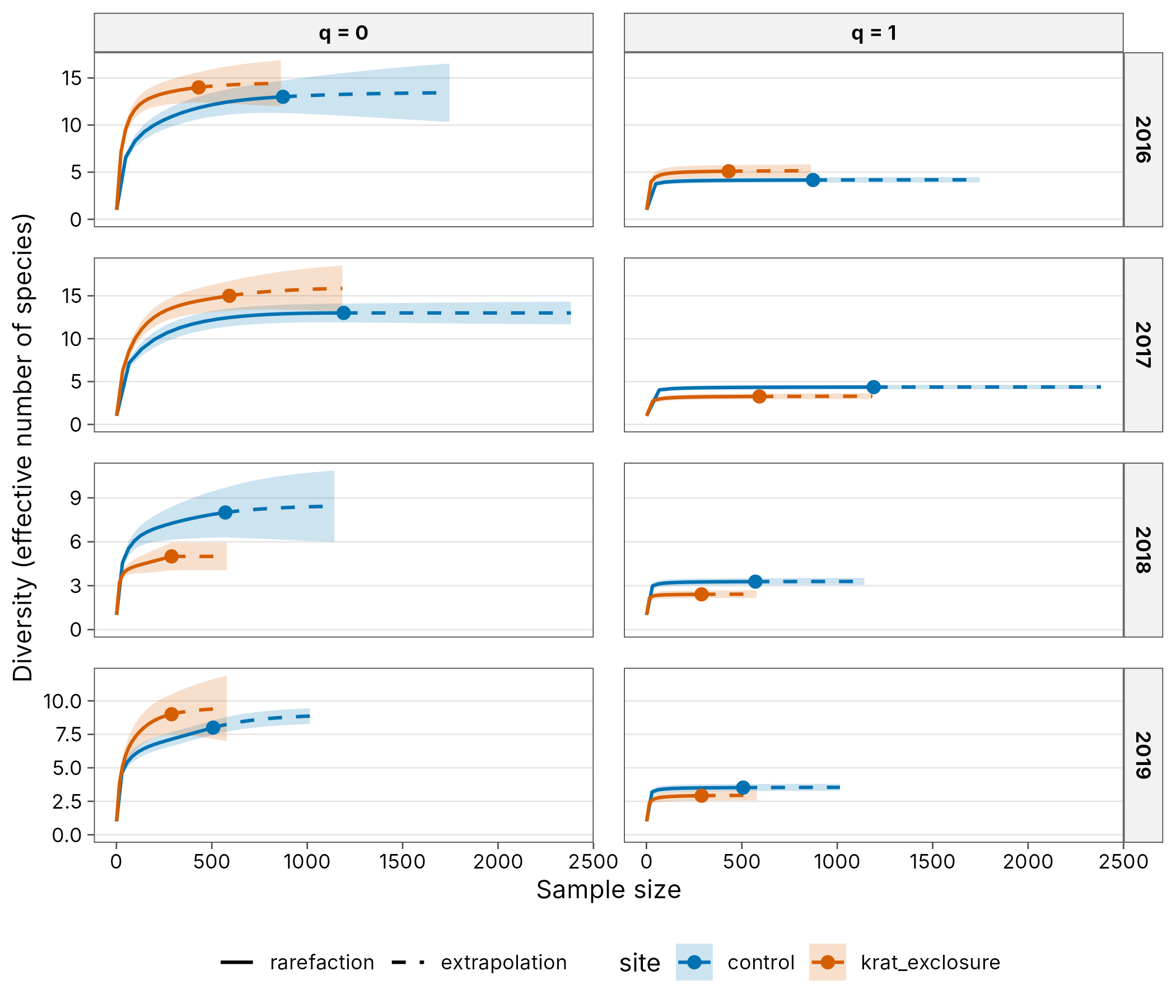
Plot-level diversity and a mixed model
Each plot is visited every year, so plot is a random effect. The coverage-standardised Shannon diversity of each plot-year is modelled against treatment and year, weighted by inverse variance. Plot-years with a single species have a standard error of zero and no finite weight, so they are dropped; weights are rescaled to a mean of one.
std <- div_standardise(rodents, q = 1, nboot = 100)
shannon <- std |>
  tidy() |>
  add_site_data(plots) |>
  filter(!is.na(weight))
shannon
#> # A tibble: 70 x 13
#>    site         q     m method    coverage estimate std.error conf.low conf.high
#>    <chr>    <dbl> <dbl> <chr>        <dbl>    <dbl>     <dbl>    <dbl>     <dbl>
#>  1 P02-2016     1  25.8 rarefact~    0.955     3.28     0.328    2.64       3.92
#>  2 P02-2017     1  48.8 rarefact~    0.955     2.75     0.394    1.97       3.52
#>  3 P02-2018     1  10.8 rarefact~    0.955     1.93     0.210    1.52       2.34
#>  4 P02-2019     1  21.7 rarefact~    0.955     2.00     0.244    1.52       2.48
#>  5 P03-2016     1  33.6 rarefact~    0.955     4.64     0.475    3.71       5.57
#>  6 P03-2017     1 103.  extrapol~    0.955     2.52     0.505    1.53       3.51
#>  7 P03-2018     1  10.7 rarefact~    0.964     1.13     0.126    0.879      1.37
#>  8 P03-2019     1  55.3 extrapol~    0.955     2.22     0.437    1.36       3.07
#>  9 P04-2016     1  64.4 rarefact~    0.955     3.90     0.359    3.19       4.60
#> 10 P04-2017     1  35.9 rarefact~    0.955     3.87     0.256    3.37       4.37
#> # i 60 more rows
#> # i 4 more variables: weight <dbl>, plot <int>, year <int>, treatment <fct>
library(lme4)
fit <- lmer(estimate ~ treatment + factor(year) + (1 | plot),
  data = shannon, weights = weight / mean(weight)
)
summary(fit)$coefficients
#>                           Estimate Std. Error    t value
#> (Intercept)              3.3119021  0.1993840 16.6106741
#> treatmentkrat_exclosure -0.5957986  0.2052048 -2.9034335
#> factor(year)2017        -0.1681186  0.2041168 -0.8236391
#> factor(year)2018        -0.8883447  0.1915441 -4.6378077
#> factor(year)2019        -1.0851290  0.1922227 -5.6451670
ggplot(shannon, aes(factor(year), estimate,
  colour = treatment,
  group = interaction(treatment, plot)
)) +
  geom_pointrange(aes(ymin = conf.low, ymax = conf.high),
    size = 0.25,
    position = position_dodge(width = 0.8)
  ) +
  scale_colour_tidydiversity() +
  labs(
    x = "Year", y = "Shannon diversity (effective number of species)",
    colour = "Treatment"
  ) +
  theme_tidydiversity()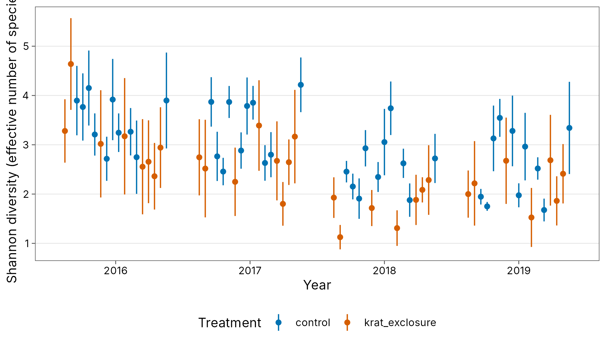
In these years, Shannon diversity on kangaroo rat exclosures is lower than on controls, with a confidence interval for the treatment effect that excludes zero:
confint(fit, parm = "treatmentkrat_exclosure", method = "Wald")
#>                              2.5 %     97.5 %
#> treatmentkrat_exclosure -0.9979926 -0.1936045
Excluding the three Dipodomys species removes part of the community outright, and the remaining assemblage is dominated by the desert pocket mouse Chaetodipus penicillatus, so the effective number of species falls. Diversity also declined on both treatments from 2016 to 2019.
Beta diversity
Multi-site Sorensen dissimilarity among plots within each treatment and year, split into turnover and nestedness.
multi <- beta_multi(rodents, .by = c(treatment, year))
multi
#> # A tibble: 8 x 6
#>   treatment       year n_sites turnover nestedness total
#>   <fct>          <int>   <int>    <dbl>      <dbl> <dbl>
#> 1 krat_exclosure  2016       8    0.6       0.0757 0.676
#> 2 krat_exclosure  2017       8    0.551     0.0777 0.629
#> 3 krat_exclosure  2018       8    0.261     0.314  0.575
#> 4 krat_exclosure  2019       8    0.410     0.252  0.662
#> 5 control         2016      10    0.45      0.127  0.577
#> 6 control         2017      10    0.547     0.0849 0.632
#> 7 control         2018      10    0.446     0.159  0.605
#> 8 control         2019      10    0.319     0.317  0.636
autoplot(multi, xlab = "Treatment")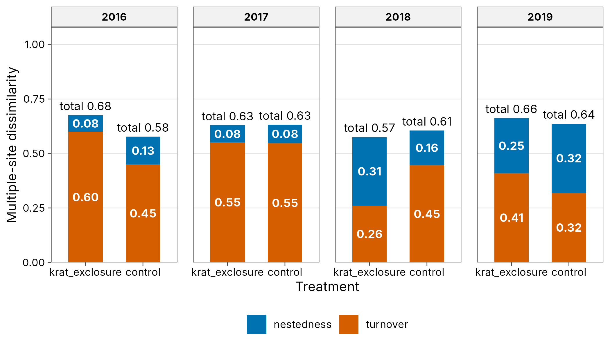
Reporting
div_table(div_estimate(filter(pooled, year == 2019), nboot = 100),
  digits = 1, output = "kable",
  caption = "Asymptotic diversity by treatment, 2019"
)| site | Order q | Observed | Estimate [95% CI] |
|---|---|---|---|
| control | 0 | 8.0 | 9.0 [8.5, 9.8] |
| control | 1 | 3.5 | 3.6 [3.5, 3.8] |
| control | 2 | 2.8 | 2.9 [2.8, 3.1] |
| krat_exclosure | 0 | 9.0 | 9.5 [9.0, 22.4] |
| krat_exclosure | 1 | 2.9 | 3.0 [2.9, 3.4] |
| krat_exclosure | 2 | 1.9 | 2.0 [1.9, 2.2] |
References
Brown, J. H., Valone, T. J. and Curtin, C. G. (1997). Reorganization of an arid ecosystem in response to recent climate change. PNAS 94: 9729-9733.
Ernest, S. K. M., Yenni, G. M., Allington, G., et al. (2018). The Portal Project: a long-term study of a Chihuahuan desert ecosystem. bioRxiv. https://doi.org/10.1101/332783