
Every plot that autoplot() draws, using
png_ants: real ant bait data from the Mt Wilhelm
elevational gradient, Papua New Guinea. Each entry has three tabs: the
plot, the tidy table behind it, and the code. All plots use the
colour-blind-safe Okabe-Ito palette and
theme_tidydiversity() by default; see the publication figures article for
customisation.
Maps are in the companion package tidymapr; see its Gallery.
library(tidydiversity)
library(dplyr)
library(ggplot2)
set.seed(1)
wet <- filter(png_ants, season == "wet")
Rarefaction and extrapolation by sample size
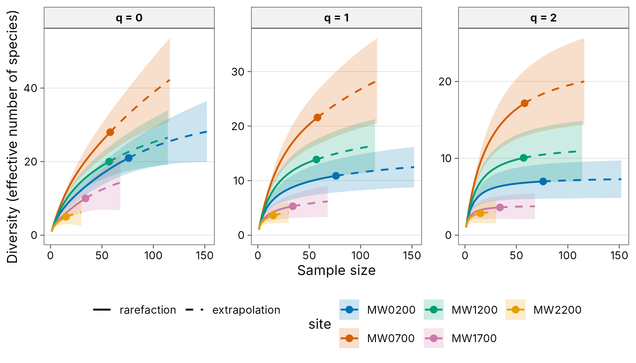
curves
#> # A tibble: 570 x 8
#>    site       q     m method      diversity coverage lower upper
#>    <chr>  <dbl> <dbl> <chr>           <dbl>    <dbl> <dbl> <dbl>
#>  1 MW0200     0     1 rarefaction      1       0.132  1     1.00
#>  2 MW0200     0     5 rarefaction      3.92    0.445  3.57  4.27
#>  3 MW0200     0     9 rarefaction      5.90    0.585  5.14  6.65
#>  4 MW0200     0    13 rarefaction      7.44    0.655  6.34  8.54
#>  5 MW0200     0    17 rarefaction      8.75    0.695  7.37 10.1
#>  6 MW0200     0    21 rarefaction      9.93    0.721  8.30 11.6
#>  7 MW0200     0    25 rarefaction     11.0     0.740  9.16 12.9
#>  8 MW0200     0    29 rarefaction     12.0     0.754  9.97 14.1
#>  9 MW0200     0    33 rarefaction     13.0     0.766 10.7  15.3
#> 10 MW0200     0    38 rarefaction     14.1     0.780 11.7  16.6
#> # i 560 more rows
curves <- div_rarefy(wet, nboot = 50)
autoplot(curves)
Rarefaction and extrapolation by sample coverage
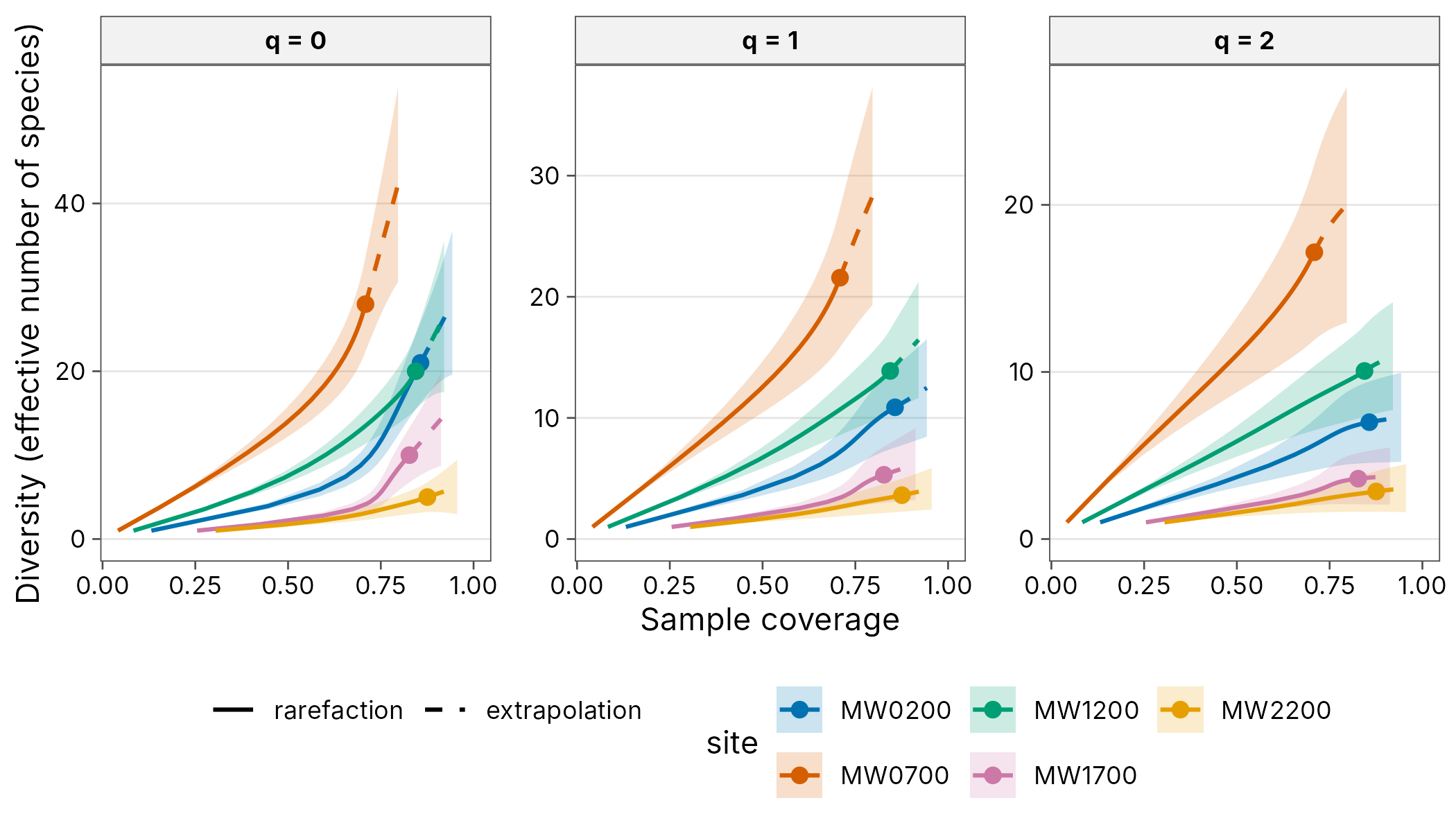
curves
#> # A tibble: 570 x 8
#>    site       q     m method      diversity coverage lower upper
#>    <chr>  <dbl> <dbl> <chr>           <dbl>    <dbl> <dbl> <dbl>
#>  1 MW0200     0     1 rarefaction      1       0.132  1     1.00
#>  2 MW0200     0     5 rarefaction      3.92    0.445  3.56  4.28
#>  3 MW0200     0     9 rarefaction      5.90    0.585  5.09  6.70
#>  4 MW0200     0    13 rarefaction      7.44    0.655  6.24  8.64
#>  5 MW0200     0    17 rarefaction      8.75    0.695  7.20 10.3
#>  6 MW0200     0    21 rarefaction      9.93    0.721  8.07 11.8
#>  7 MW0200     0    25 rarefaction     11.0     0.740  8.88 13.2
#>  8 MW0200     0    29 rarefaction     12.0     0.754  9.64 14.4
#>  9 MW0200     0    33 rarefaction     13.0     0.766 10.4  15.6
#> 10 MW0200     0    38 rarefaction     14.1     0.780 11.2  17.1
#> # i 560 more rows
curves <- div_rarefy(wet, nboot = 50)
autoplot(curves, x = "coverage")
Curves for several groups
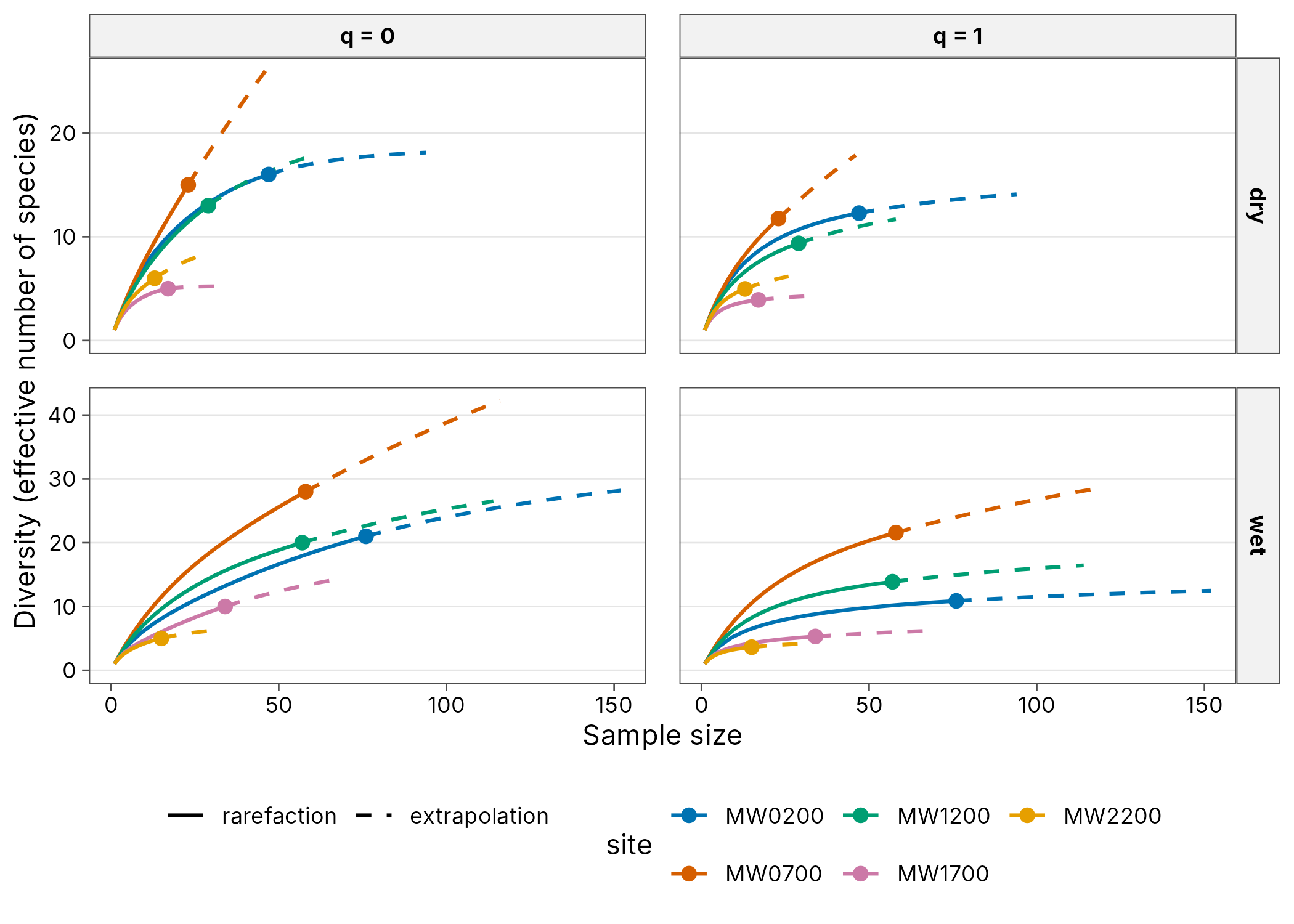
grouped
#> # A tibble: 740 x 9
#>    season site       q     m method      diversity coverage lower upper
#>    <chr>  <chr>  <dbl> <dbl> <chr>           <dbl>    <dbl> <dbl> <dbl>
#>  1 dry    MW0200     0     1 rarefaction      1      0.0814    NA    NA
#>  2 dry    MW0200     0     3 rarefaction      2.76   0.220     NA    NA
#>  3 dry    MW0200     0     6 rarefaction      4.94   0.377     NA    NA
#>  4 dry    MW0200     0     8 rarefaction      6.14   0.457     NA    NA
#>  5 dry    MW0200     0    11 rarefaction      7.67   0.549     NA    NA
#>  6 dry    MW0200     0    13 rarefaction      8.55   0.596     NA    NA
#>  7 dry    MW0200     0    16 rarefaction      9.70   0.652     NA    NA
#>  8 dry    MW0200     0    18 rarefaction     10.4    0.682     NA    NA
#>  9 dry    MW0200     0    21 rarefaction     11.3    0.720     NA    NA
#> 10 dry    MW0200     0    23 rarefaction     11.8    0.741     NA    NA
#> # i 730 more rows
grouped <- div_rarefy(png_ants, q = c(0, 1), .by = season)
autoplot(grouped)
Diversity at equal coverage
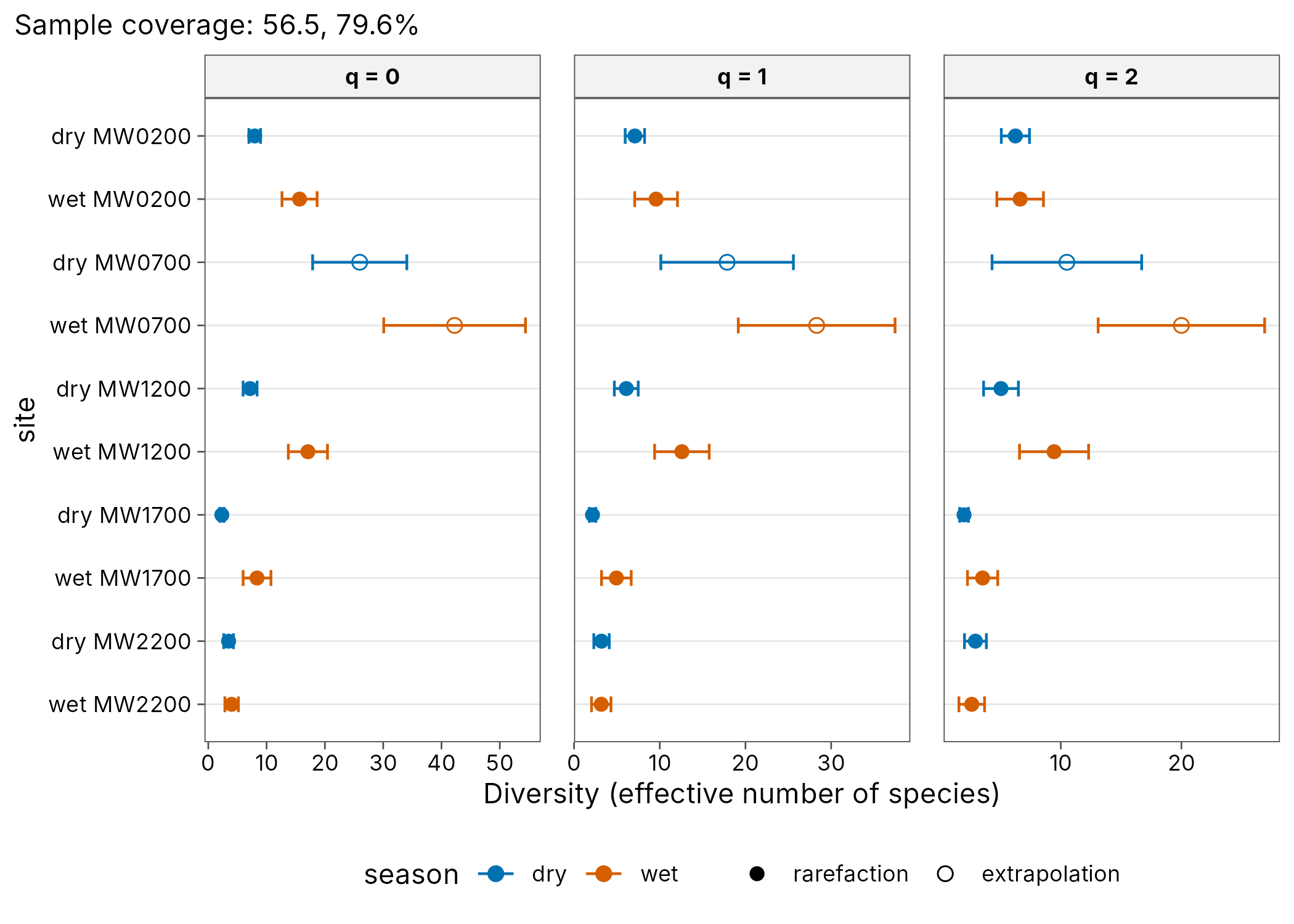
std
#> # A tibble: 30 x 10
#>    season site       q     m method        coverage diversity    se lower upper
#>    <chr>  <chr>  <dbl> <dbl> <chr>            <dbl>     <dbl> <dbl> <dbl> <dbl>
#>  1 dry    MW0200     0  11.6 rarefaction      0.565      7.96 0.510  6.96  8.96
#>  2 dry    MW0200     1  11.6 rarefaction      0.565      7.10 0.577  5.97  8.23
#>  3 dry    MW0200     2  11.6 rarefaction      0.565      6.24 0.596  5.07  7.40
#>  4 wet    MW0200     0  45.1 rarefaction      0.796     15.7  1.54  12.6  18.7
#>  5 wet    MW0200     1  45.1 rarefaction      0.796      9.57 1.27   7.08 12.1
#>  6 wet    MW0200     2  45.1 rarefaction      0.796      6.63 0.985  4.70  8.56
#>  7 dry    MW0700     0  46.0 extrapolation    0.565     26.0  4.12  17.9  34.1
#>  8 dry    MW0700     1  46.0 extrapolation    0.565     17.9  3.95  10.1  25.6
#>  9 dry    MW0700     2  46.0 extrapolation    0.565     10.5  3.16   4.30 16.7
#> 10 wet    MW0700     0 116   extrapolation    0.796     42.2  6.20  30.1  54.4
#> # i 20 more rows
std <- div_standardise(png_ants, .by = season, nboot = 50)
autoplot(std)
Observed and asymptotic diversity
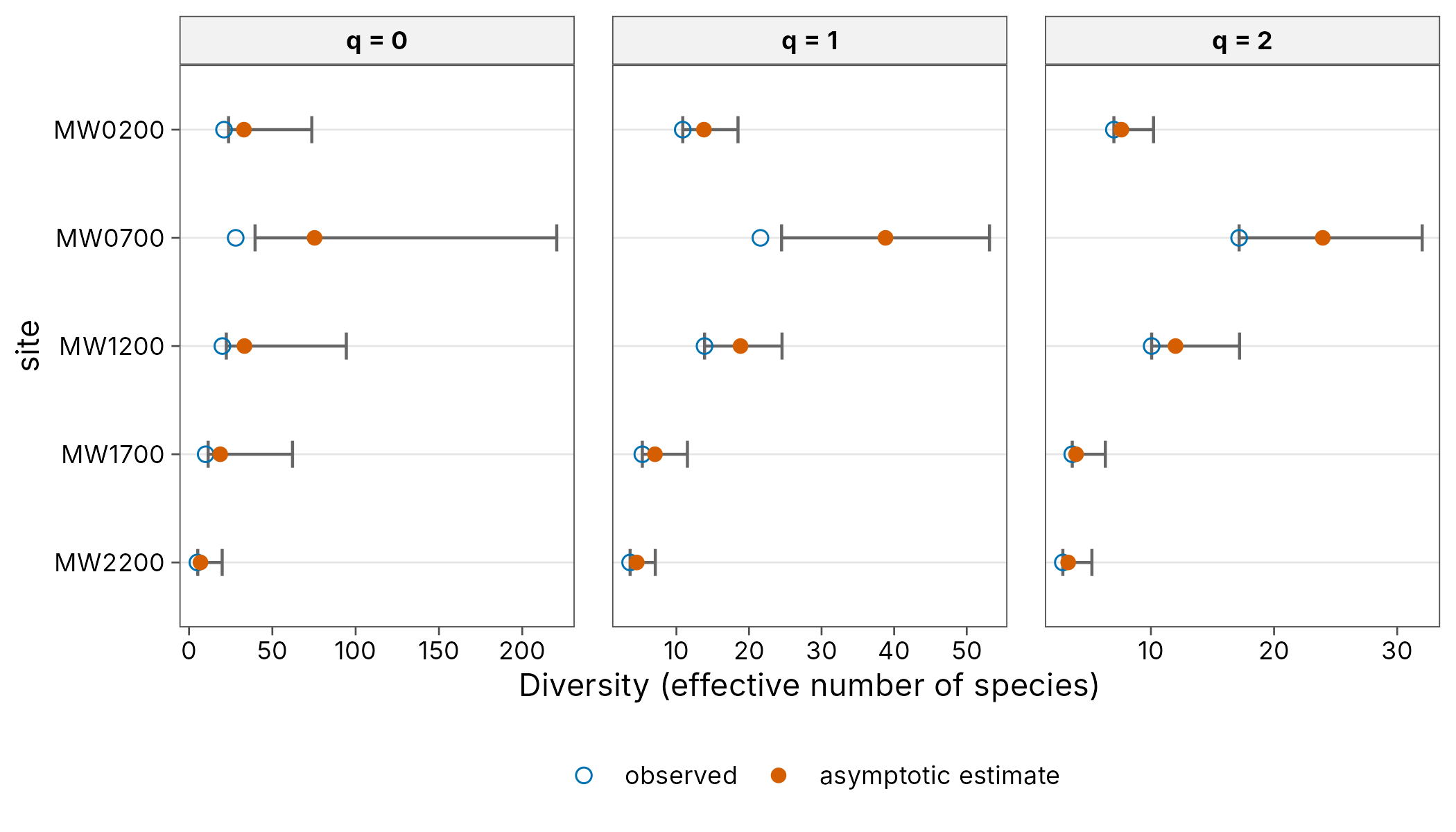
est
#> # A tibble: 15 x 7
#>    site       q observed estimate     se lower  upper
#>    <chr>  <dbl>    <dbl>    <dbl>  <dbl> <dbl>  <dbl>
#>  1 MW0200     0    21       32.9  10.5   23.7   73.7
#>  2 MW0200     1    10.9     13.8   2.40  10.9   18.5
#>  3 MW0200     2     6.99     7.6   1.33   6.99  10.2
#>  4 MW0700     0    28       75.3  38.8   39.6  221.
#>  5 MW0700     1    21.6     38.8   7.31  24.5   53.1
#>  6 MW0700     2    17.2     24.0   4.12  17.2   32.0
#>  7 MW1200     0    20       33.3  14.3   22.4   94.4
#>  8 MW1200     1    13.9     18.8   2.92  13.9   24.6
#>  9 MW1200     2    10.1     12     2.65  10.1   17.2
#> 10 MW1700     0    10       18.7   9.94  11.5   62.1
#> 11 MW1700     1     5.30     7.05  2.28   5.30  11.5
#> 12 MW1700     2     3.61     3.92  1.21   3.61   6.30
#> 13 MW2200     0     5        6.87  2.69   5.23  19.9
#> 14 MW2200     1     3.62     4.54  1.30   3.62   7.09
#> 15 MW2200     2     2.85     3.28  0.983  2.85   5.21
est <- div_estimate(wet, nboot = 50)
autoplot(est)
Hill diversity profile
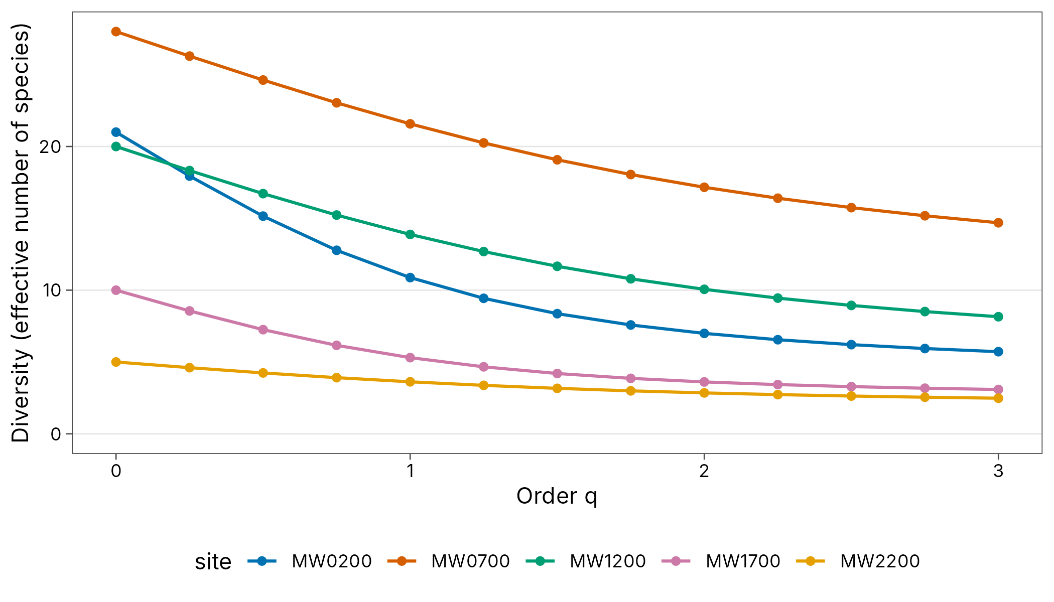
profile
#> # A tibble: 65 x 4
#>    site       q     n diversity
#>    <chr>  <dbl> <dbl>     <dbl>
#>  1 MW0200  0       76     21
#>  2 MW0200  0.25    76     17.9
#>  3 MW0200  0.5     76     15.2
#>  4 MW0200  0.75    76     12.8
#>  5 MW0200  1       76     10.9
#>  6 MW0200  1.25    76      9.43
#>  7 MW0200  1.5     76      8.36
#>  8 MW0200  1.75    76      7.58
#>  9 MW0200  2       76      6.99
#> 10 MW0200  2.25    76      6.55
#> # i 55 more rowsDiversity along a gradient
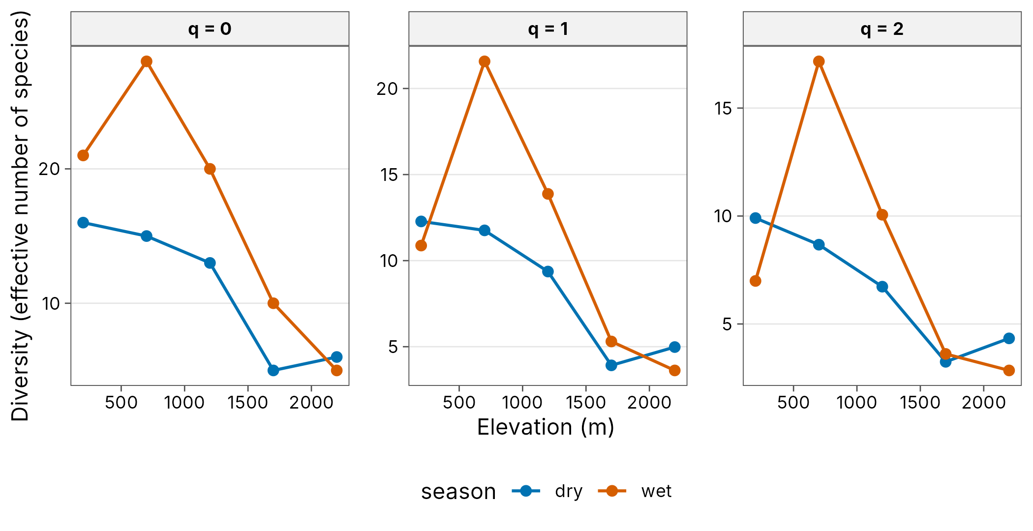
hill
#> # A tibble: 30 x 6
#>    season elevation site       q     n diversity
#>    <chr>      <int> <chr>  <dbl> <dbl>     <dbl>
#>  1 dry          200 MW0200     0    47     16
#>  2 dry          200 MW0200     1    47     12.3
#>  3 dry          200 MW0200     2    47      9.91
#>  4 wet          200 MW0200     0    76     21
#>  5 wet          200 MW0200     1    76     10.9
#>  6 wet          200 MW0200     2    76      6.99
#>  7 dry          700 MW0700     0    23     15
#>  8 dry          700 MW0700     1    23     11.8
#>  9 dry          700 MW0700     2    23      8.67
#> 10 wet          700 MW0700     0    58     28
#> # i 20 more rowsSample coverage
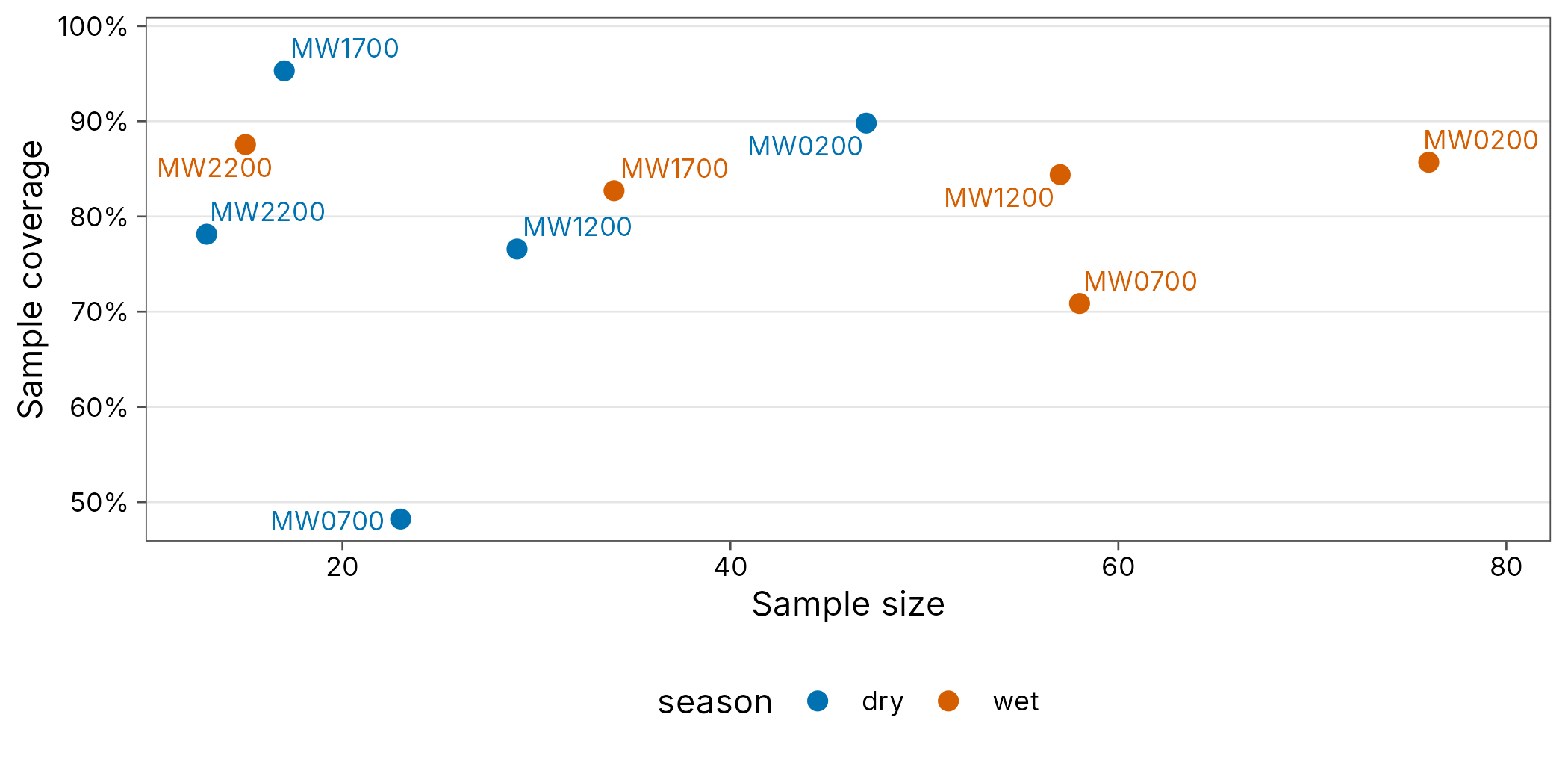
cov
#> # A tibble: 10 x 7
#>    season site       n s_obs    f1    f2 coverage
#>    <chr>  <chr>  <dbl> <int> <int> <int>    <dbl>
#>  1 dry    MW0200    47    16     5     5    0.898
#>  2 wet    MW0200    76    21    11     5    0.857
#>  3 dry    MW0700    23    15    12     1    0.482
#>  4 wet    MW0700    58    28    17     3    0.709
#>  5 dry    MW1200    29    13     7     3    0.766
#>  6 wet    MW1200    57    20     9     3    0.844
#>  7 dry    MW1700    17     5     1     2    0.953
#>  8 wet    MW1700    34    10     6     2    0.827
#>  9 dry    MW2200    13     6     3     1    0.781
#> 10 wet    MW2200    15     5     2     1    0.876
cov <- div_coverage(png_ants, .by = season)
autoplot(cov)
Pairwise beta diversity heatmap
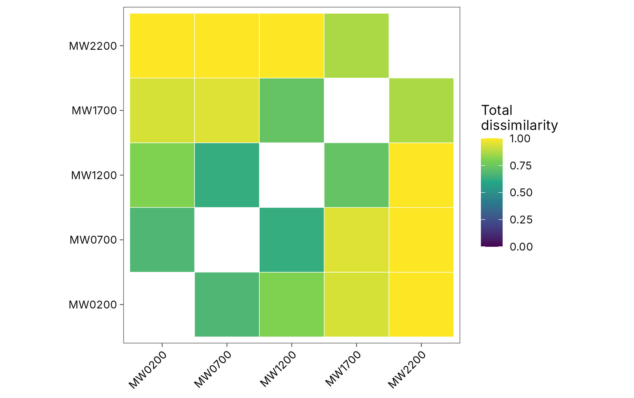
pair
#> # A tibble: 10 x 5
#>    site_1 site_2 turnover nestedness total
#>    <chr>  <chr>     <dbl>      <dbl> <dbl>
#>  1 MW0200 MW0700    0.619    0.0544  0.673
#>  2 MW0200 MW1200    0.8      0.00488 0.805
#>  3 MW0200 MW1700    0.9      0.0355  0.935
#>  4 MW0200 MW2200    1        0       1
#>  5 MW0700 MW1200    0.55     0.075   0.625
#>  6 MW0700 MW1700    0.9      0.0474  0.947
#>  7 MW0700 MW2200    1        0       1
#>  8 MW1200 MW1700    0.6      0.133   0.733
#>  9 MW1200 MW2200    1        0       1
#> 10 MW1700 MW2200 0.8 0.0667 0.867Multiple-site beta partition
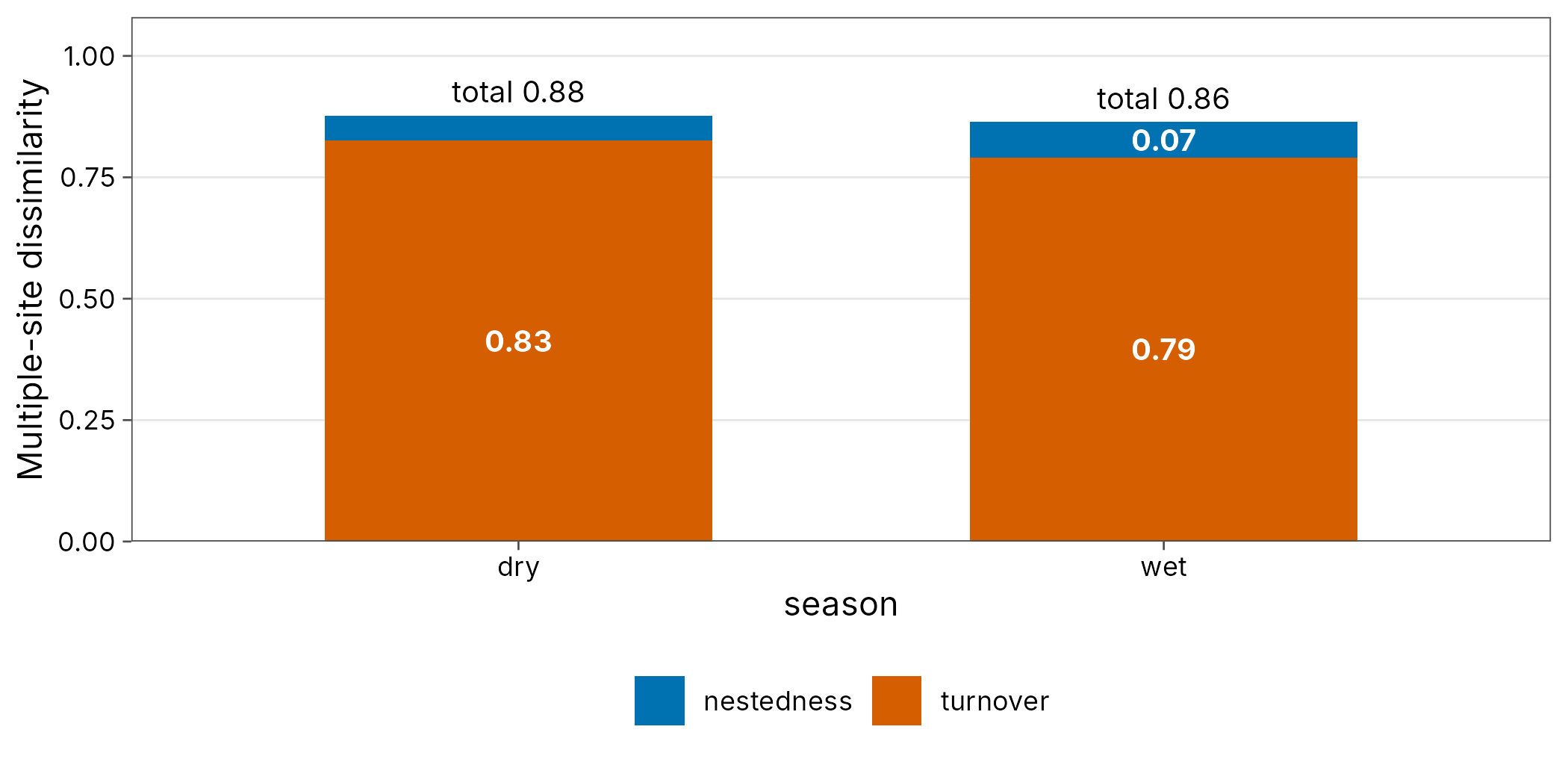
multi
#> # A tibble: 2 x 5
#>   season n_sites turnover nestedness total
#>   <chr>    <int>    <dbl>      <dbl> <dbl>
#> 1 dry          5    0.827     0.0507 0.877
#> 2 wet          5    0.790     0.0737 0.864
multi <- beta_multi(png_ants, .by = season)
autoplot(multi)
Distance decay
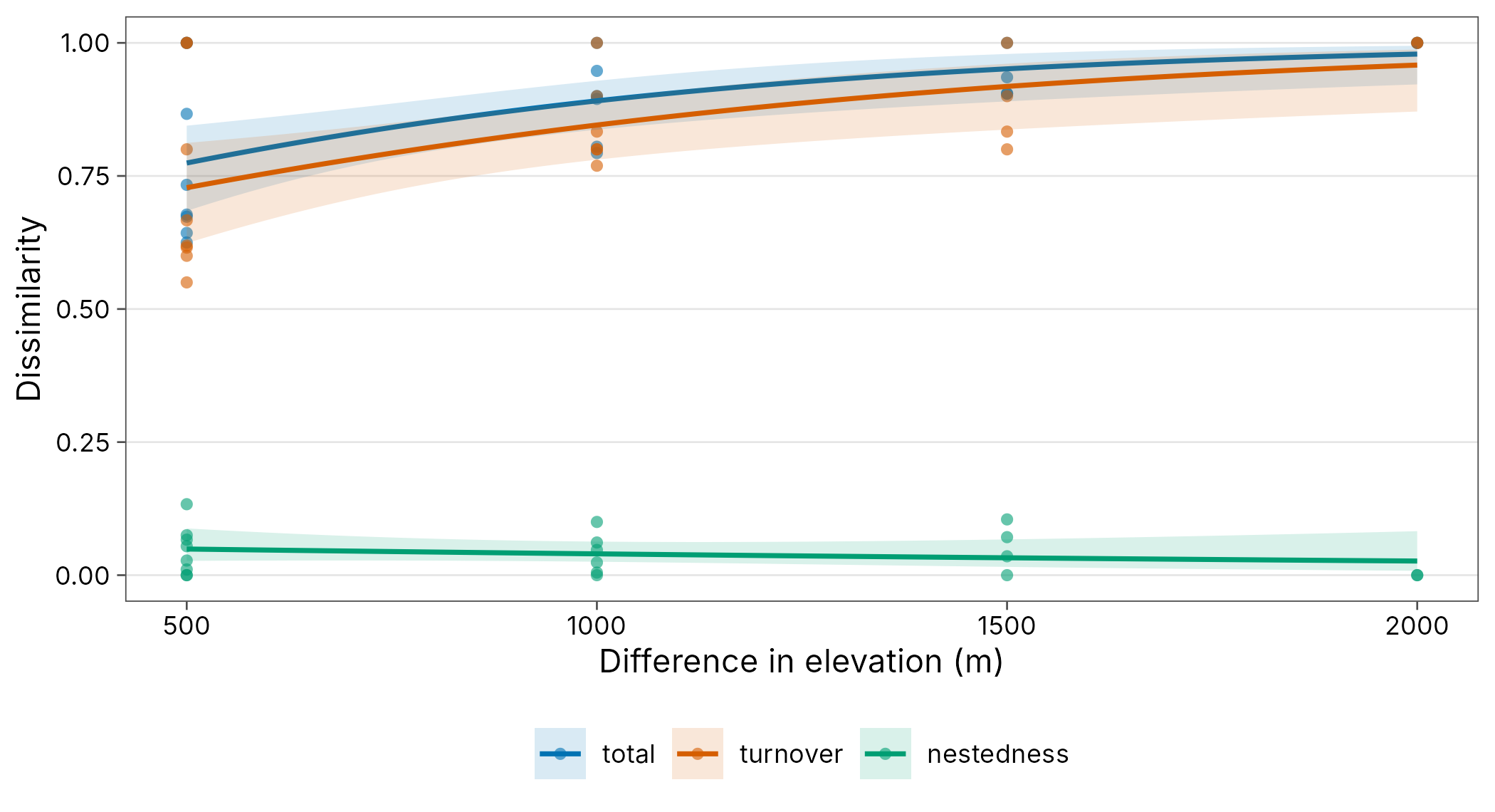
decay
#> # A tibble: 20 x 9
#>    season site_1 site_2 turnover nestedness total gradient_1 gradient_2 distance
#>    <chr>  <chr>  <chr>     <dbl>      <dbl> <dbl>      <int>      <int>    <dbl>
#>  1 dry    MW0200 MW0700    0.667    0.0108  0.677        200        700      500
#>  2 dry    MW0200 MW1200    0.769    0.0239  0.793        200       1200     1000
#>  3 dry    MW0200 MW1700    0.8      0.105   0.905        200       1700     1500
#>  4 dry    MW0200 MW2200    1        0       1            200       2200     2000
#>  5 dry    MW0700 MW1200    0.615    0.0275  0.643        700       1200      500
#>  6 dry    MW0700 MW1700    0.8      0.1     0.9          700       1700     1000
#>  7 dry    MW0700 MW2200    0.833    0.0714  0.905        700       2200     1500
#>  8 dry    MW1200 MW1700    1        0       1           1200       1700      500
#>  9 dry    MW1200 MW2200    0.833    0.0614  0.895       1200       2200     1000
#> 10 dry    MW1700 MW2200    1        0       1           1700       2200      500
#> 11 wet    MW0200 MW0700    0.619    0.0544  0.673        200        700      500
#> 12 wet    MW0200 MW1200    0.8      0.00488 0.805        200       1200     1000
#> 13 wet    MW0200 MW1700    0.9      0.0355  0.935        200       1700     1500
#> 14 wet    MW0200 MW2200    1        0       1            200       2200     2000
#> 15 wet    MW0700 MW1200    0.55     0.075   0.625        700       1200      500
#> 16 wet    MW0700 MW1700    0.9      0.0474  0.947        700       1700     1000
#> 17 wet    MW0700 MW2200    1        0       1            700       2200     1500
#> 18 wet    MW1200 MW1700    0.6      0.133   0.733       1200       1700      500
#> 19 wet    MW1200 MW2200    1        0       1           1200       2200     1000
#> 20 wet    MW1700 MW2200    0.8      0.0667  0.867       1700       2200      500
set.seed(1)
beta_decay_model(decay)
#> # A tibble: 2 x 10
#>   season model    component n_pairs     a       b half_distance pseudo_r2    aic
#>   <chr>  <chr>    <chr>       <int> <dbl>   <dbl>         <dbl>     <dbl>  <dbl>
#> 1 dry    exponen~ total          10 0.257 7.50e-4          924.     0.143  -9.21
#> 2 wet    exponen~ total          10 0.897 2.36e-3          293.     0.694 -17.6
#> # i 1 more variable: p.value <dbl>
decay <- beta_decay(png_ants, elevation, .by = season)
autoplot(decay, xlab = "Difference in elevation (m)")
beta_decay_model(decay)
Pairwise Hill dissimilarity
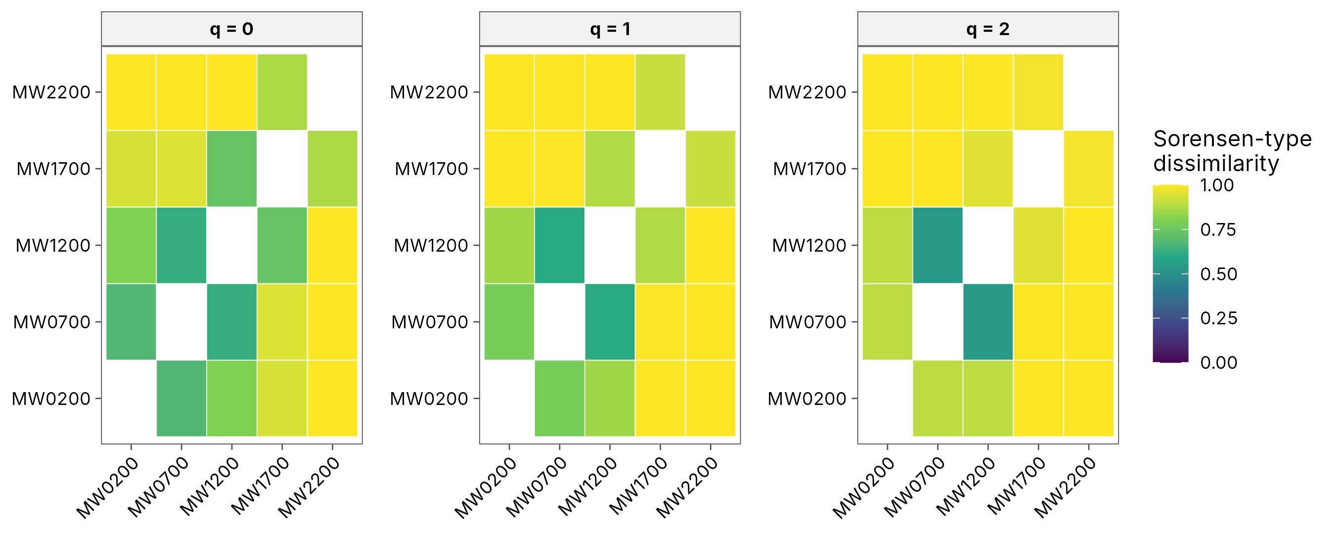
hp
#> # A tibble: 30 x 10
#>    site_1 site_2     q gamma alpha  beta dis_sorensen dis_jaccard
#>    <chr>  <chr>  <dbl> <dbl> <dbl> <dbl>        <dbl>       <dbl>
#>  1 MW0200 MW0700     0    41  24.5  1.67        0.673       0.805
#>  2 MW0200 MW1200     0    37  20.5  1.80        0.805       0.892
#>  3 MW0200 MW1700     0    30  15.5  1.94        0.935       0.967
#>  4 MW0200 MW2200     0    26  13    2           1           1
#>  5 MW0700 MW1200     0    39  24    1.62        0.625       0.769
#>  6 MW0700 MW1700     0    37  19    1.95        0.947       0.973
#>  7 MW0700 MW2200     0    33  16.5  2           1           1
#>  8 MW1200 MW1700     0    26  15    1.73        0.733       0.846
#>  9 MW1200 MW2200     0    25  12.5  2           1           1
#> 10 MW1700 MW2200     0    14   7.5  1.87        0.867       0.929
#> # i 20 more rows
#> # i 2 more variables: dis_turnover_sorensen <dbl>, dis_turnover_jaccard <dbl>
wet <- dplyr::filter(png_ants, season == "wet")
hp <- beta_hill_pair(wet, abundance = workers)
autoplot(hp)
Coverage-standardised beta diversity
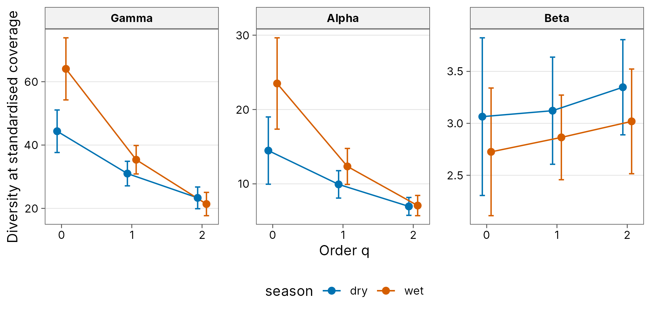
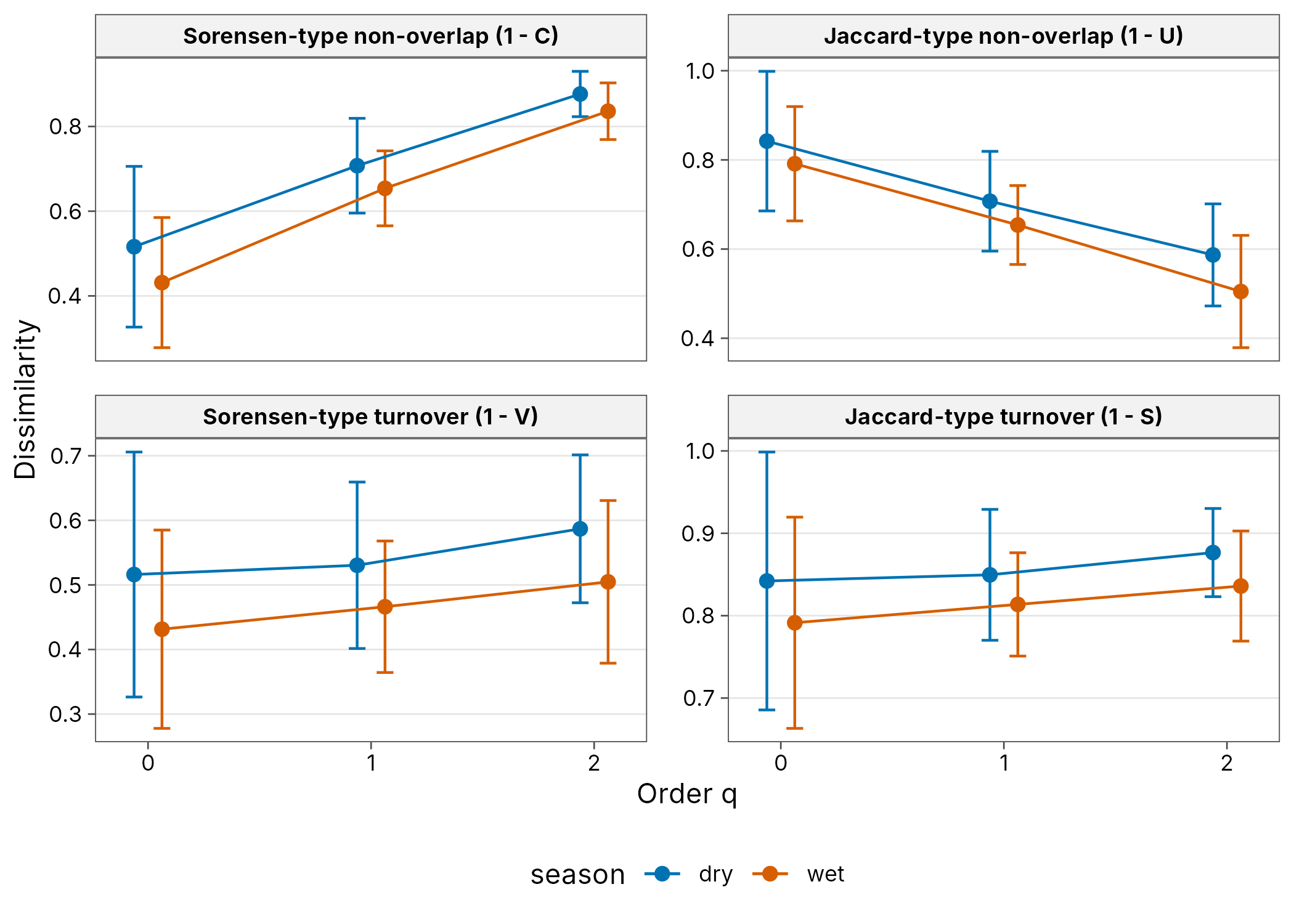
hb[c("season", "q", "gamma", "alpha", "beta", "beta_lower", "beta_upper")]
#> # A tibble: 6 x 7
#>   season     q gamma alpha  beta beta_lower beta_upper
#>   <chr>  <dbl> <dbl> <dbl> <dbl>      <dbl>      <dbl>
#> 1 dry        0  44.4 14.5   3.06       2.31       3.82
#> 2 dry        1  31.0  9.93  3.12       2.61       3.64
#> 3 dry        2  23.3  6.97  3.35       2.89       3.81
#> 4 wet        0  64.1 23.5   2.73       2.11       3.34
#> 5 wet        1  35.4 12.3   2.86       2.46       3.27
#> 6 wet 2 21.4 7.08 3.02 2.52 3.52Greyscale for print
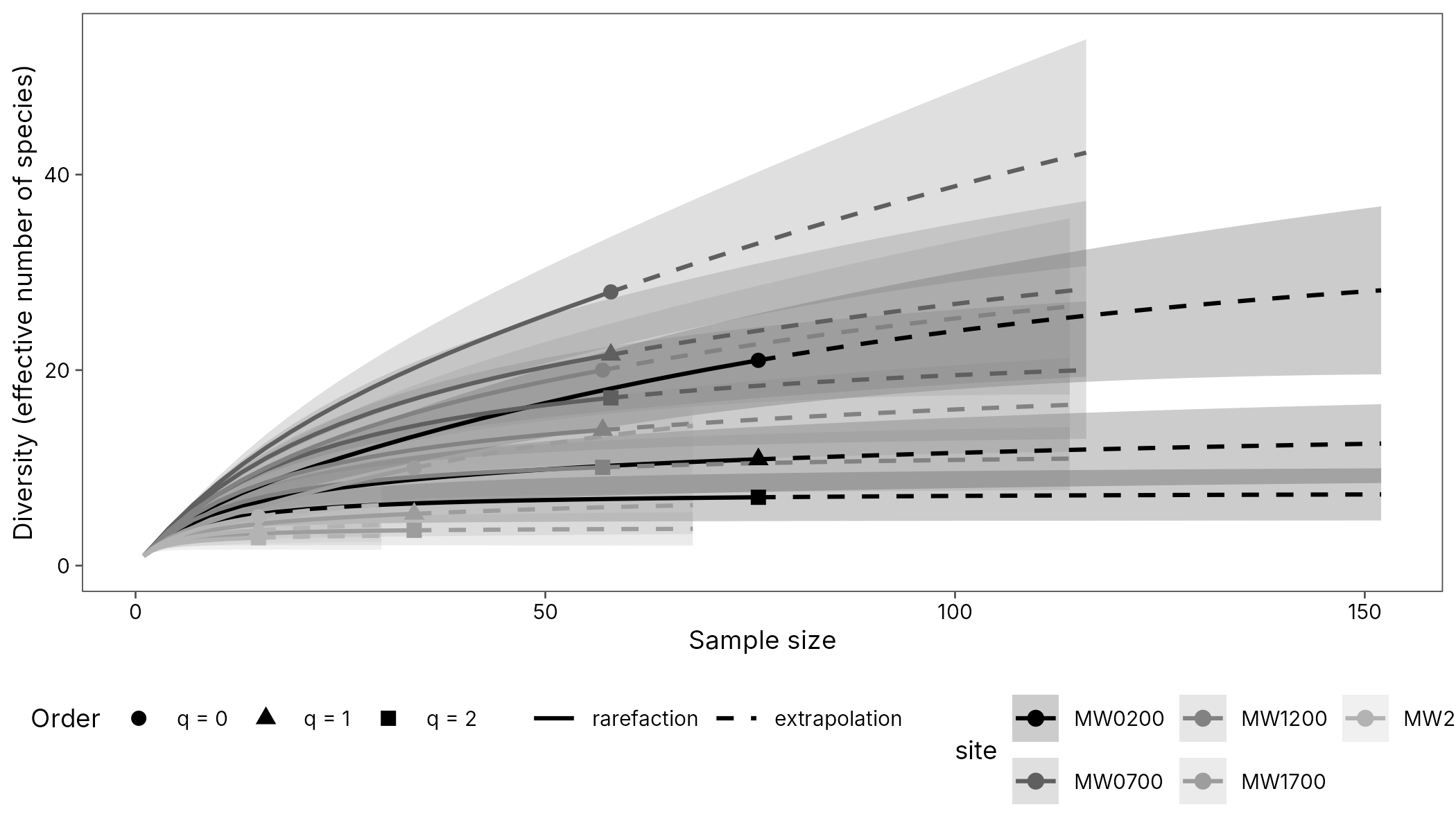
curves
#> # A tibble: 570 x 8
#>    site       q     m method      diversity coverage lower upper
#>    <chr>  <dbl> <dbl> <chr>           <dbl>    <dbl> <dbl> <dbl>
#>  1 MW0200     0     1 rarefaction      1       0.132  1     1.00
#>  2 MW0200     0     5 rarefaction      3.92    0.445  3.56  4.28
#>  3 MW0200     0     9 rarefaction      5.90    0.585  5.09  6.70
#>  4 MW0200     0    13 rarefaction      7.44    0.655  6.24  8.64
#>  5 MW0200     0    17 rarefaction      8.75    0.695  7.20 10.3
#>  6 MW0200     0    21 rarefaction      9.93    0.721  8.07 11.8
#>  7 MW0200     0    25 rarefaction     11.0     0.740  8.88 13.2
#>  8 MW0200     0    29 rarefaction     12.0     0.754  9.64 14.4
#>  9 MW0200     0    33 rarefaction     13.0     0.766 10.4  15.6
#> 10 MW0200     0    38 rarefaction     14.1     0.780 11.2  17.1
#> # i 560 more rows
autoplot(curves, palette = "grey", facet = FALSE,
  theme = theme_tidydiversity(base_size = 9, grid = "none"))
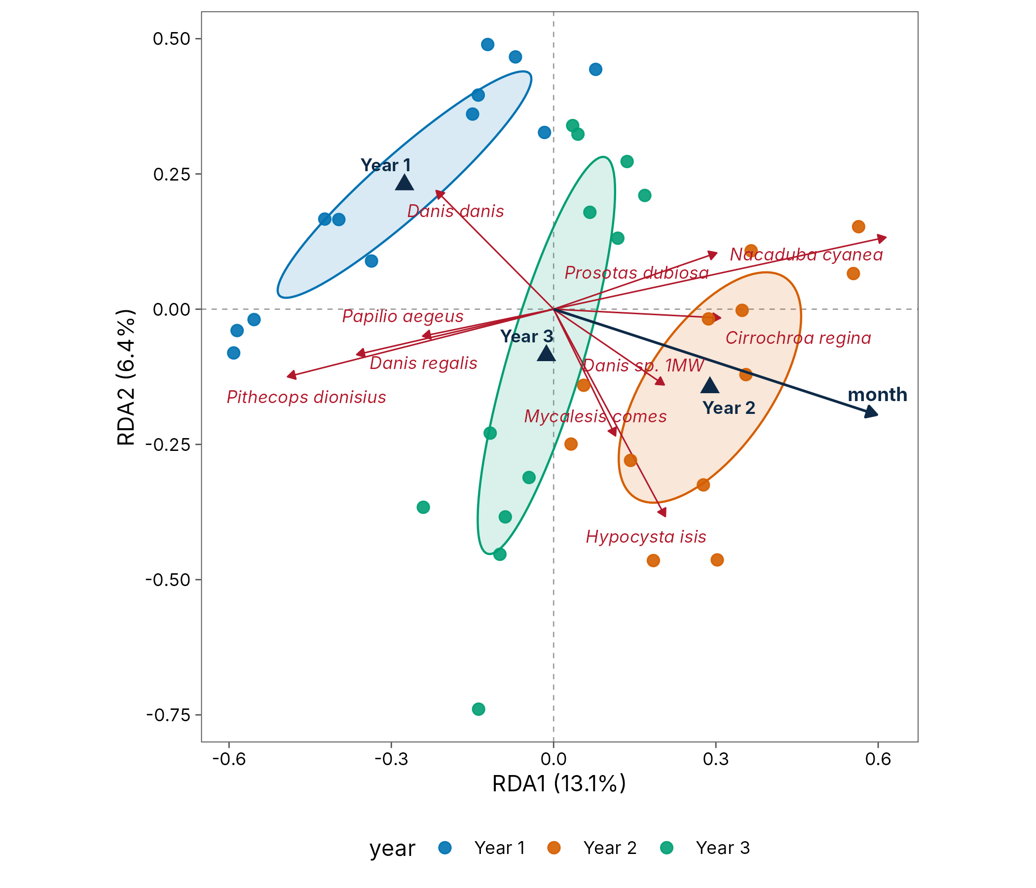
Ordination triplot
An RDA of the Wanang butterflies constrained by year and month: sites, the ten best-fitting species (red arrows), the month gradient (dark arrow), year centroids and ellipses for each year.
Shared species: Venn diagram
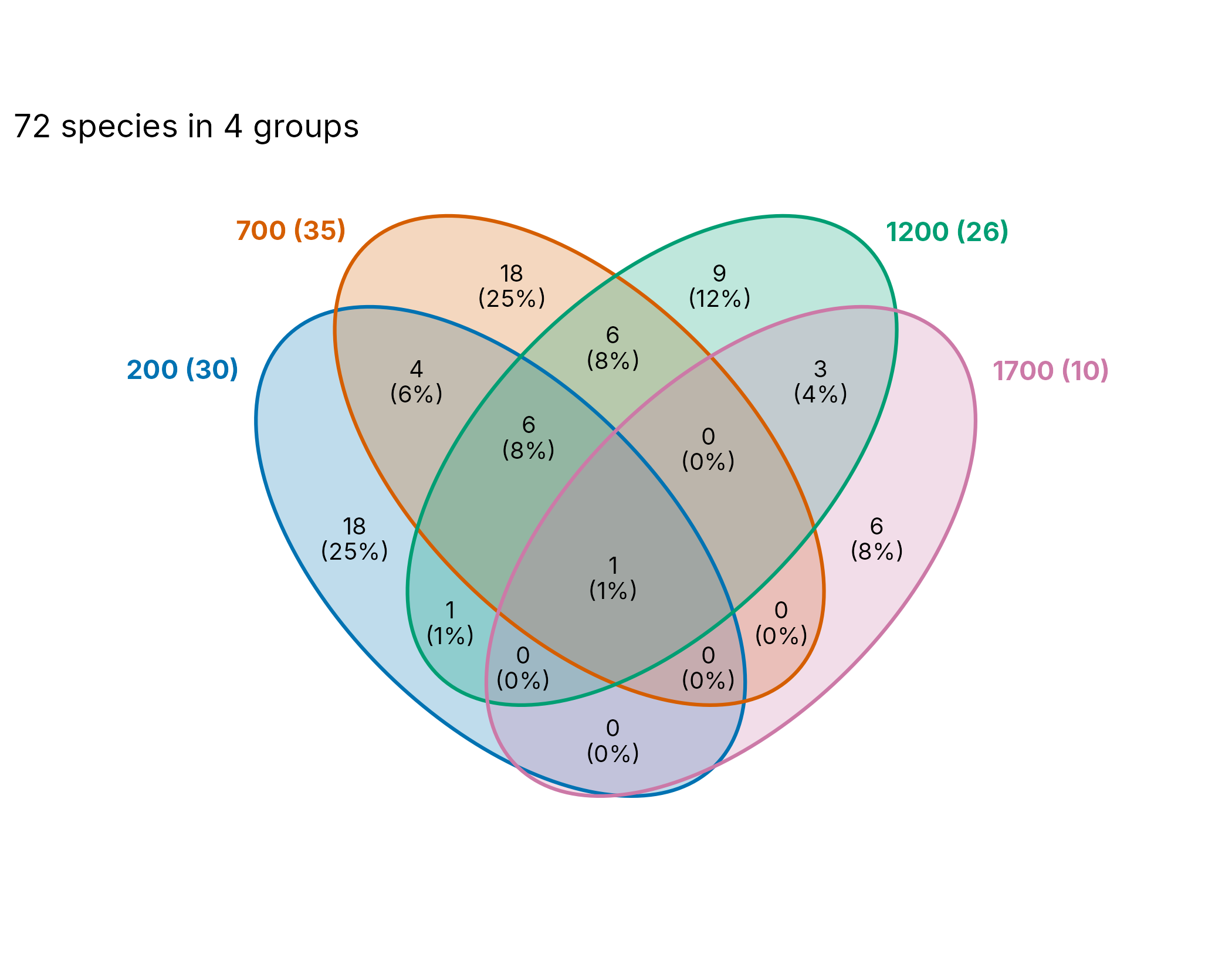
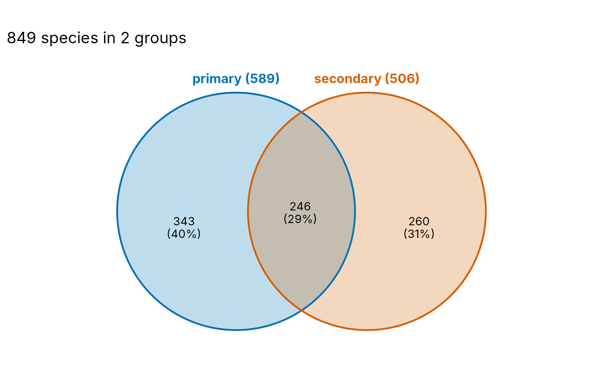
plot_venn() counts the species found in each combination
of two to four groups. Here, ant species at four elevations on Mt
Wilhelm.
Phylogenetic diversity
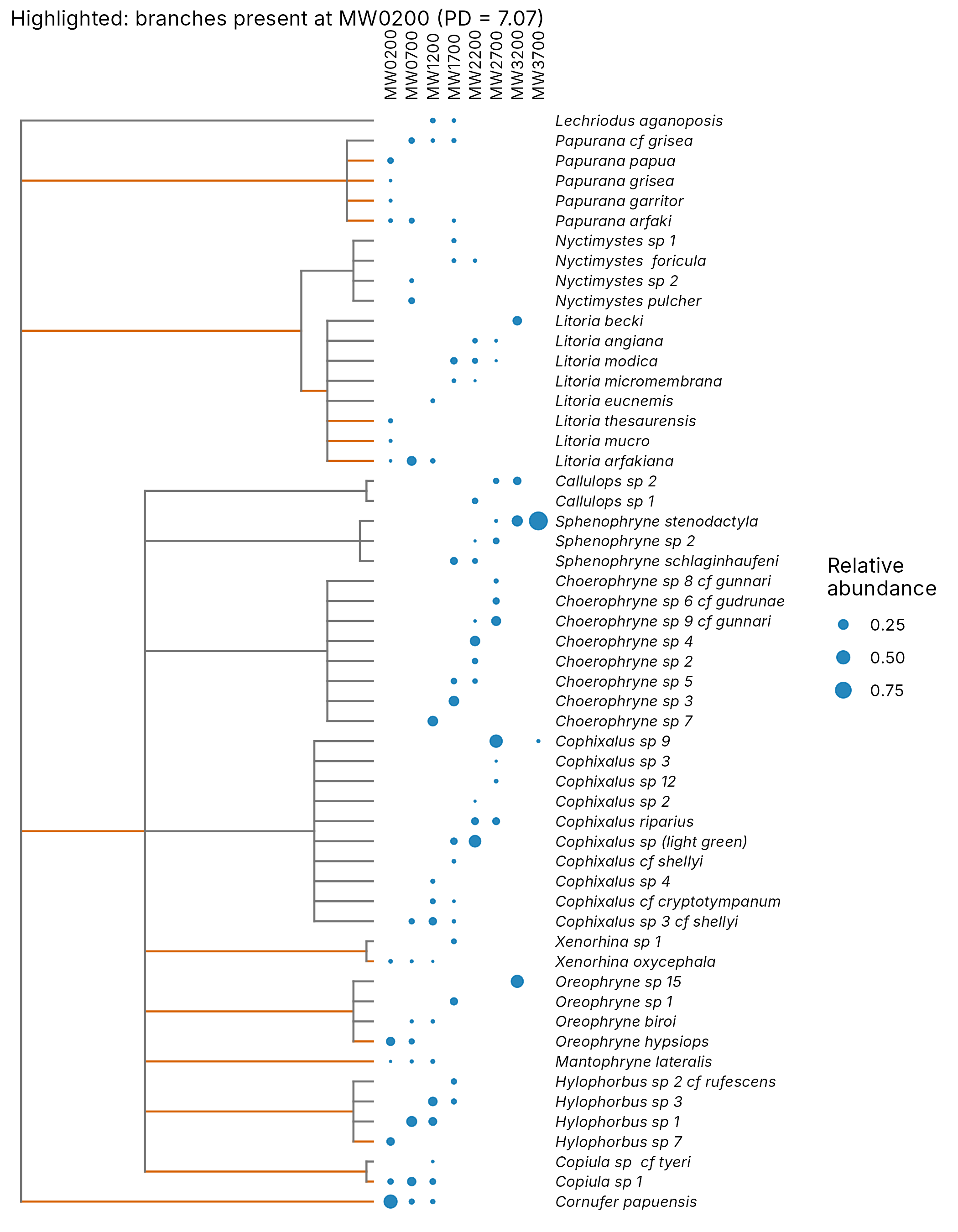
plot_phylo() draws the tree with each species’ relative
abundance per site. The coloured branches lead to the frogs found at 200
m: their total length is Faith’s PD for that site. The tree here is a
taxonomic tree (family, genus, species) with Grafen branch lengths; use
a dated phylogeny where one exists.
frogs <- mutate(png_frogs,
  genus = sub(" .*", "", scientific_name),
  tip = gsub(" ", "_", scientific_name)
)
tax <- distinct(as.data.frame(frogs[c("family", "genus", "tip")]))
tax[] <- lapply(tax, factor)
tree <- ape::compute.brlen(ape::as.phylo(~ family / genus / tip, data = tax))
plot_phylo(tree, frogs, species = tip, abundance = abundance, highlight = "MW0200")
Functional trait space
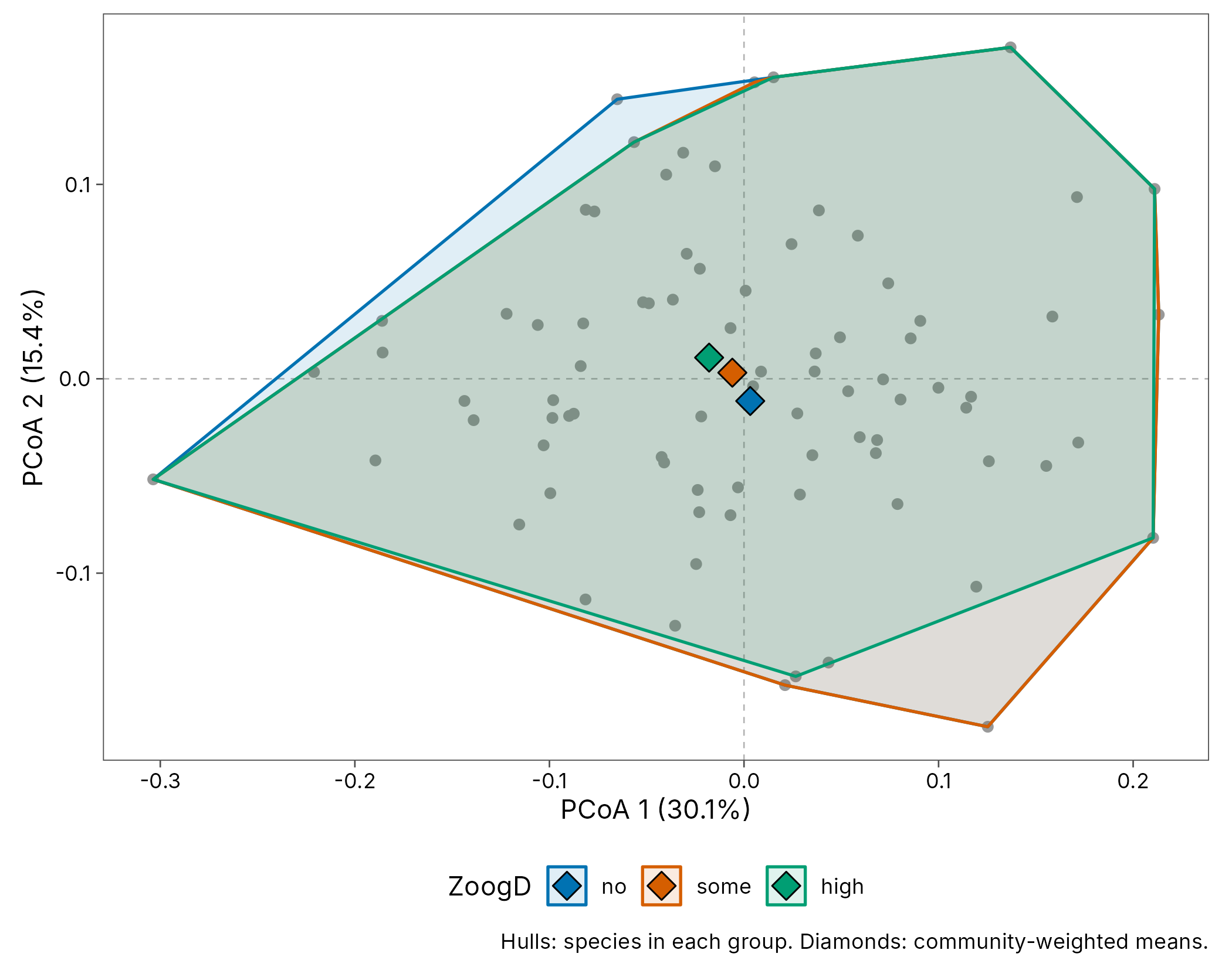
plot_trait_space() places the alpine plants of the
aravo data in a PCoA of Gower trait distances. Each hull
encloses the species found under one level of zoogenic disturbance (its
area is the two-dimensional functional richness) and the diamonds are
cover-weighted mean positions.
aravo <- data_aravo()
plot_trait_space(aravo$traits, aravo$community, group = ZoogD, abundance = cover)