Case study: trees on Barro Colorado Island

The 50 ha forest dynamics plot on Barro Colorado Island, Panama, is one of the best known tree censuses in the world. The BCI dataset in vegan holds counts of 225 tree species with a stem diameter of at least 10 cm in fifty 1 ha subplots, and BCI.env holds habitat type, environmental heterogeneity and coordinates for each subplot.

Source and licence. Condit et al. (2002), distributed with vegan (Oksanen et al.; licence GPL-2). The data are loaded from vegan at run time and are not redistributed with tidydiversity.

library(tidydiversity)
library(dplyr)
library(ggplot2)
set.seed(2026)

Tidy the data

data(BCI, BCI.env, package = "vegan")
env <- tibble::tibble(
  site = sprintf("ha%02d", seq_len(nrow(BCI))),
  habitat = BCI.env$Habitat,
  env_het = BCI.env$EnvHet,
  x = BCI.env$UTM.EW - min(BCI.env$UTM.EW),
  y = BCI.env$UTM.NS - min(BCI.env$UTM.NS)
)
trees <- community_long(bind_cols(site = env$site, BCI), cols = -site)
trees
#> # A community: 50 sites, 225 species, 21,457 individuals
#>    site  species                 abundance
#>    <chr> <chr>                       <int>
#>  1 ha01  Alchornea.costaricensis         2
#>  2 ha01  Alseis.blackiana               25
#>  3 ha01  Annona.spraguei                 1
#>  4 ha01  Apeiba.glabra                  13
#>  5 ha01  Apeiba.tibourbou                2
#>  6 ha01  Astronium.graveolens            6
#>  7 ha01  Beilschmiedia.pendula           4
#>  8 ha01  Brosimum.alicastrum             5
#>  9 ha01  Casearia.arborea                1
#> 10 ha01  Casearia.sylvestris             2
#> # i 4,529 more rows

Completeness and curves

cov <- div_coverage(trees)
summary(cov$coverage)
#>    Min. 1st Qu.  Median    Mean 3rd Qu.    Max. 
#>  0.8710  0.9097  0.9202  0.9184  0.9289  0.9470

Each hectare has about 400 trees, and coverage is between about 87% and 95%: tropical forests have many rare species, so one in every ten or so further trees would still be a species not yet recorded in that hectare. The richness curves are far from flat, while Shannon and Simpson diversity are much closer to their asymptotes.

curves <- div_rarefy(filter(trees, site %in% c(
  "ha01", "ha13", "ha25",
  "ha50"
)), nboot = 100)
autoplot(curves, ylab = "Diversity (effective number of tree species)")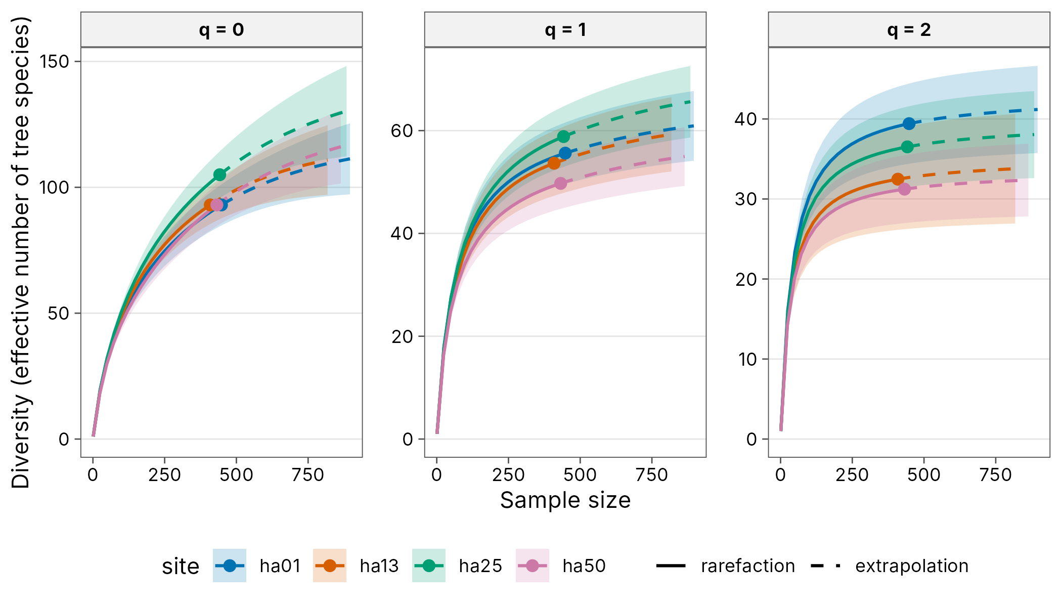

Diversity profiles

div_hill(filter(trees, site %in% c("ha01", "ha13", "ha25", "ha50")),
  q = seq(0, 3, by = 0.25)
) |>
  autoplot()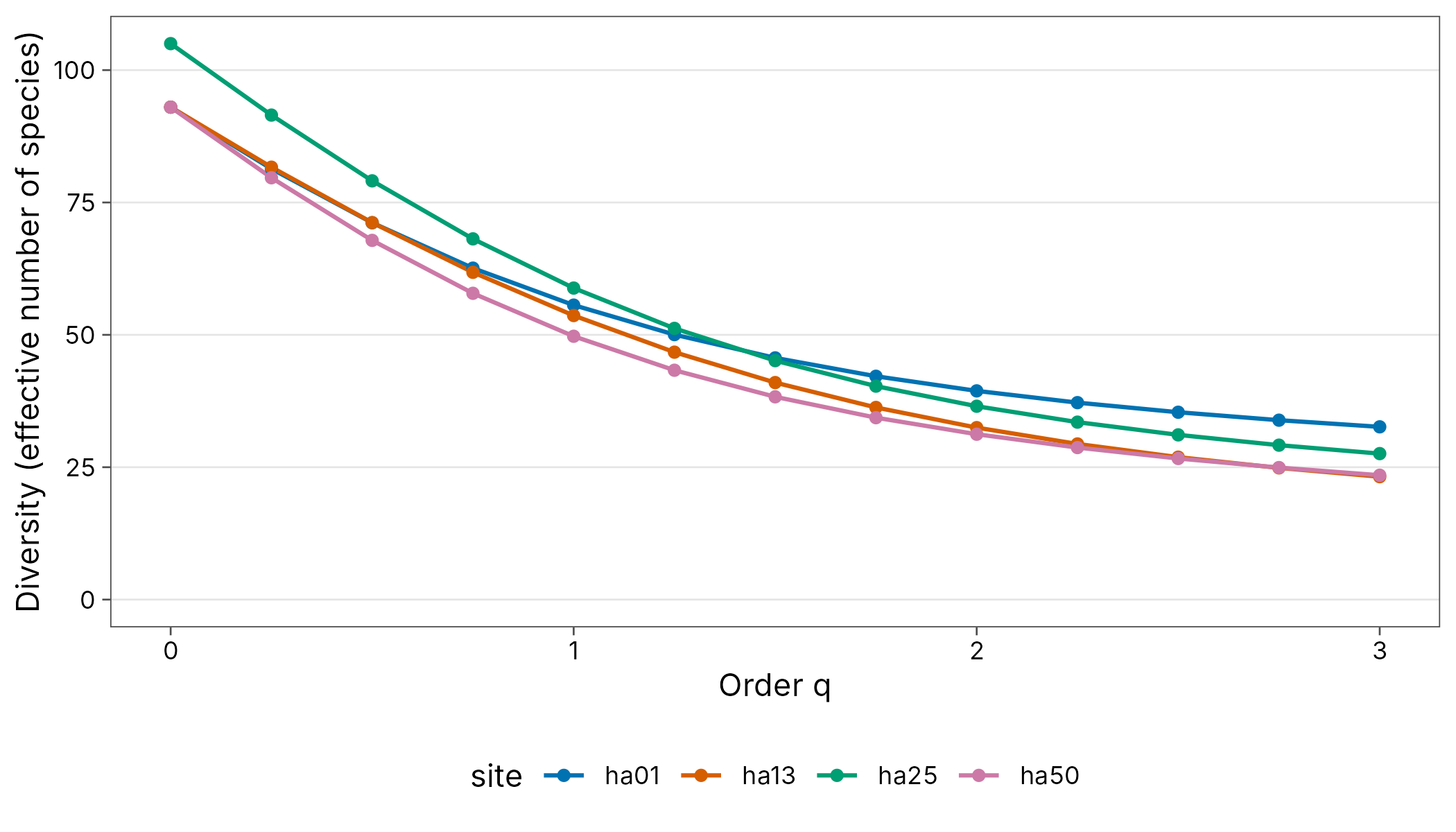

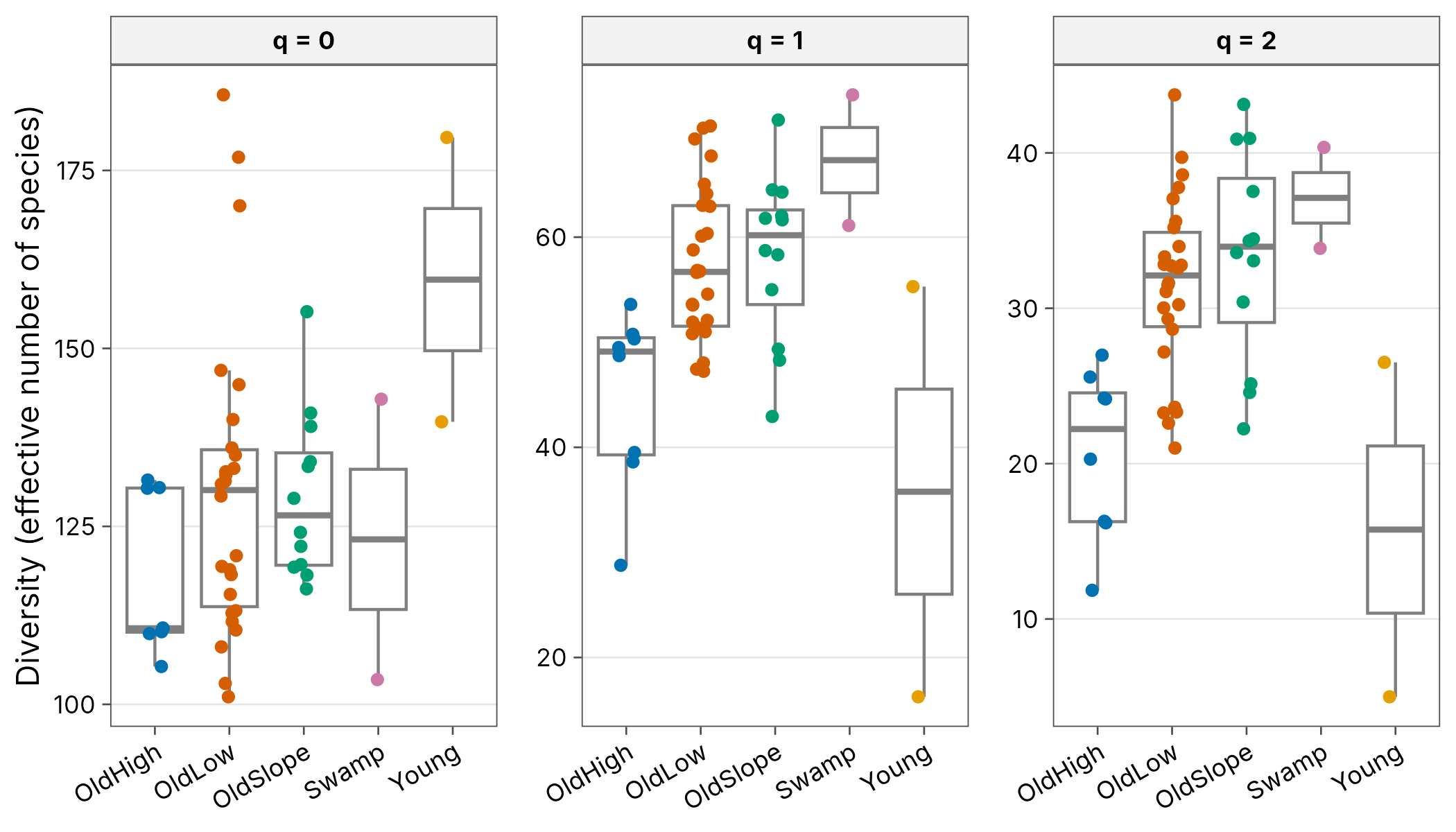
Diversity and habitat

est <- div_estimate(trees, q = c(0, 1, 2), nboot = 100) |>
  tidy() |>
  add_site_data(env)
fit <- lm(estimate ~ habitat + env_het,
  data = filter(est, q == 1),
  weights = weight
)
broom::tidy(fit, conf.int = TRUE)
#> # A tibble: 6 x 7
#>   term            estimate std.error statistic  p.value conf.low conf.high
#>   <chr>              <dbl>     <dbl>     <dbl>    <dbl>    <dbl>     <dbl>
#> 1 (Intercept)        41.2       3.37    12.2   9.72e-16    34.4       48.0
#> 2 habitatOldLow      14.0       3.39     4.14  1.57e- 4     7.20      20.9
#> 3 habitatOldSlope    13.8       3.95     3.48  1.13e- 3     5.81      21.7
#> 4 habitatSwamp       22.2       8.36     2.65  1.12e- 2     5.30      39.0
#> 5 habitatYoung      -21.6       4.43    -4.88  1.42e- 5   -30.5      -12.7
#> 6 env_het             3.34      5.93     0.563 5.76e- 1    -8.61      15.3

ggplot(est, aes(habitat, estimate, colour = habitat)) +
  geom_boxplot(outlier.shape = NA, colour = "grey50") +
  geom_jitter(width = 0.15, height = 0) +
  facet_wrap(~ paste("q =", q), scales = "free_y") +
  scale_colour_tidydiversity() +
  labs(x = NULL, y = "Diversity (effective number of species)") +
  theme_tidydiversity() +
  theme(
    legend.position = "none",
    axis.text.x = element_text(angle = 30, hjust = 1)
  )

Distance decay

Bray-Curtis dissimilarity rises slowly with the distance between hectares, and almost all of it is balanced variation (turnover) rather than abundance gradients. Passing two coordinate columns gives Euclidean distance.

decay <- trees |>
  left_join(env, by = "site") |>
  beta_decay(gradient = c(x, y), index = "bray")
autoplot(decay, xlab = "Distance between hectares (m)")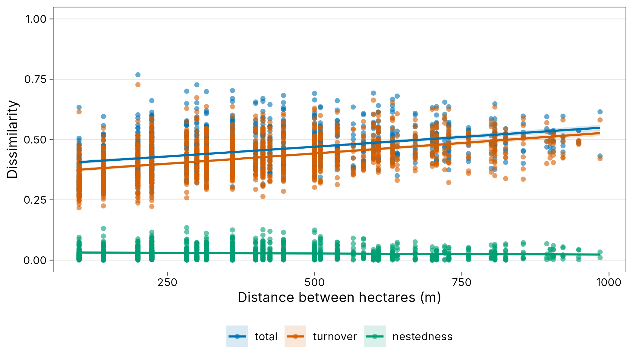

Ordination and PERMANOVA

beta_dist() turns pairwise results into a dist object for vegan.

bray <- beta_pair(trees, index = "bray")
d <- beta_dist(bray)
vegan::adonis2(d ~ habitat + env_het, data = env, permutations = 499)
#> Permutation test for adonis under reduced model
#> Permutation: free
#> Number of permutations: 499
#> 
#> vegan::adonis2(formula = d ~ habitat + env_het, data = env, permutations = 499)
#>          Df SumOfSqs     R2      F Pr(>F)   
#> Model     5   1.4830 0.2827 3.4683  0.002 **
#> Residual 44   3.7627 0.7173                 
#> Total    49   5.2457 1.0000                 
#> ---
#> Signif. codes:  0 '***' 0.001 '**' 0.01 '*' 0.05 '.' 0.1 ' ' 1

nmds <- vegan::metaMDS(d, trace = FALSE)
scores <- bind_cols(env, as.data.frame(vegan::scores(nmds)))
ggplot(scores, aes(NMDS1, NMDS2, colour = habitat)) +
  geom_point(size = 2.5) +
  coord_equal() +
  scale_colour_tidydiversity() +
  labs(colour = "Habitat") +
  theme_tidydiversity(legend_position = "right")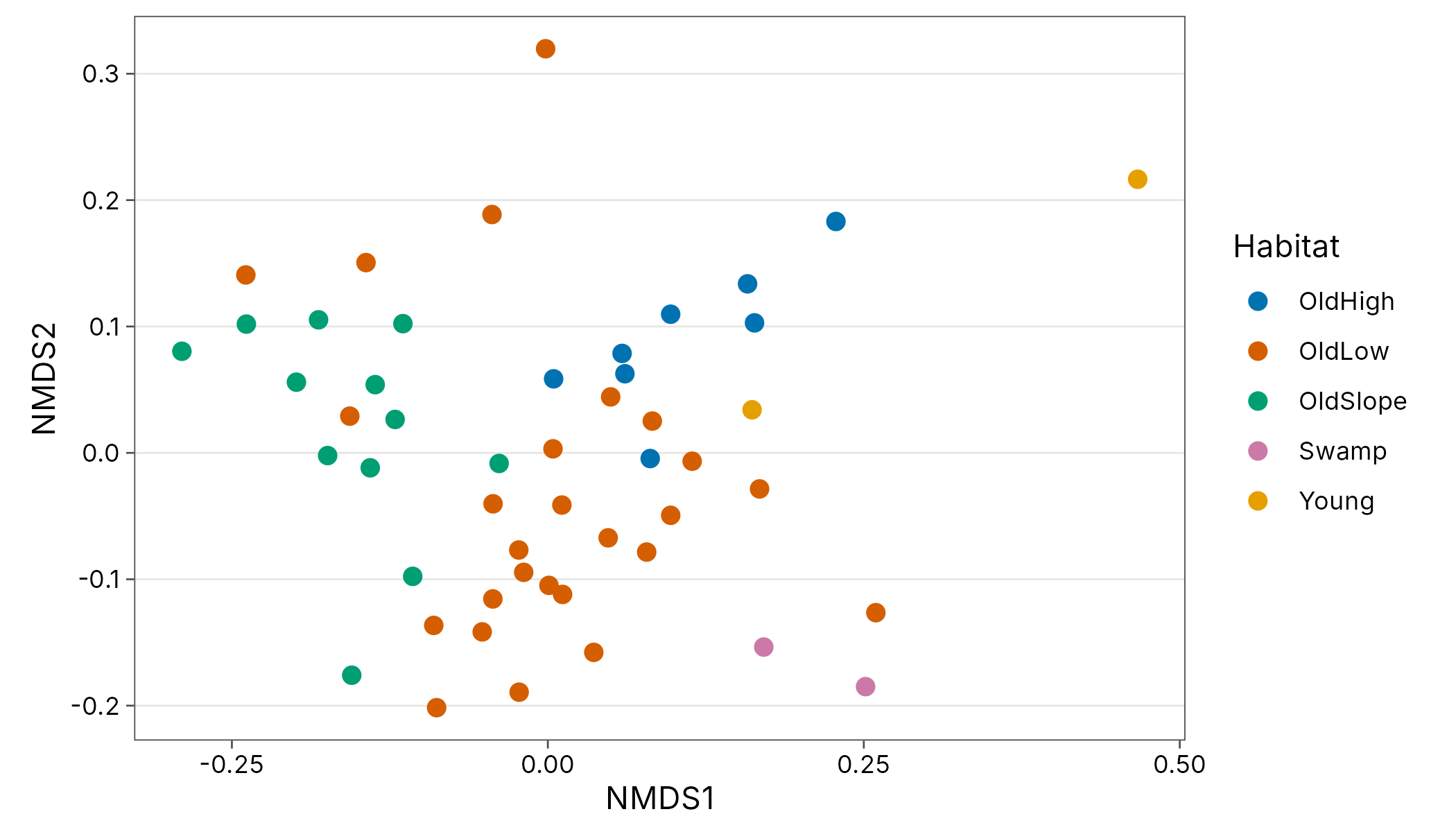

References

Condit, R., Pitman, N., Leigh, E. G., et al. (2002). Beta-diversity in tropical forest trees. Science 295: 666-669.

Oksanen, J., Simpson, G. L., Blanchet, F. G., et al. vegan: Community Ecology Package. https://CRAN.R-project.org/package=vegan