Plot tidydiversity results — autoplot-tidydiversity • tidydiversity

autoplot() methods draw a ggplot for every result type:

Usage

# S3 method for class 'td_rarefy'
autoplot(
  object,
  x = c("size", "coverage"),
  palette = "okabe_ito",
  theme = theme_tidydiversity(),
  ci = TRUE,
  facet = TRUE,
  scales = "free_y",
  ncol = NULL,
  xlab = NULL,
  ylab = y_hill,
  ...
)

# S3 method for class 'td_standardise'
autoplot(
  object,
  palette = "okabe_ito",
  theme = theme_tidydiversity(),
  ci = TRUE,
  facet = TRUE,
  scales = "free_x",
  ncol = NULL,
  xlab = NULL,
  ylab = NULL,
  ...
)

# S3 method for class 'td_beta_decay'
autoplot(
  object,
  palette = "okabe_ito",
  theme = theme_tidydiversity(),
  ci = TRUE,
  xlab = "Distance between sites",
  ylab = "Dissimilarity",
  ...
)

# S3 method for class 'td_hill'
autoplot(
  object,
  gradient = NULL,
  palette = "okabe_ito",
  theme = theme_tidydiversity(),
  facet = TRUE,
  scales = "free_y",
  ncol = NULL,
  xlab = NULL,
  ylab = y_hill,
  ...
)

# S3 method for class 'td_estimate'
autoplot(
  object,
  palette = "okabe_ito",
  theme = theme_tidydiversity(),
  ci = TRUE,
  facet = TRUE,
  scales = "free_x",
  ncol = NULL,
  xlab = y_hill,
  ylab = NULL,
  ...
)

# S3 method for class 'td_coverage'
autoplot(
  object,
  palette = "okabe_ito",
  theme = theme_tidydiversity(),
  xlab = "Sample size",
  ylab = "Sample coverage",
  labels = TRUE,
  ...
)

# S3 method for class 'td_beta_pair'
autoplot(
  object,
  component = c("total", "turnover", "nestedness"),
  theme = theme_tidydiversity(grid = "none"),
  ...
)

# S3 method for class 'td_beta_hill_pair'
autoplot(
  object,
  component = c("dis_sorensen", "dis_jaccard", "dis_turnover_sorensen",
    "dis_turnover_jaccard"),
  theme = theme_tidydiversity(grid = "none"),
  ...
)

# S3 method for class 'td_beta_multi'
autoplot(
  object,
  palette = "okabe_ito",
  theme = theme_tidydiversity(),
  xlab = NULL,
  ylab = "Multiple-site dissimilarity",
  labels = TRUE,
  digits = 2,
  ...
)

# S3 method for class 'td_beta_hill'
autoplot(
  object,
  what = c("diversity", "dissimilarity"),
  palette = "okabe_ito",
  theme = theme_tidydiversity(),
  ci = TRUE,
  xlab = "Order q",
  ylab = NULL,
  ...
)

# S3 method for class 'td_dispersion'
autoplot(object, palette = "okabe_ito", theme = theme_tidydiversity(), ...)

# S3 method for class 'td_completeness'
autoplot(
  object,
  palette = "okabe_ito",
  theme = theme_tidydiversity(),
  xlab = "Order q",
  ylab = "Sample completeness",
  ...
)

# S3 method for class 'td_evenness'
autoplot(
  object,
  palette = "okabe_ito",
  theme = theme_tidydiversity(),
  xlab = "Order q",
  ylab = "Evenness",
  ...
)

Arguments

object: A tibble returned by one of the functions above.
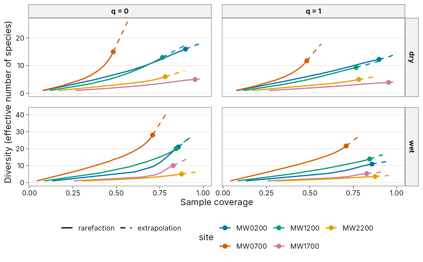
x: For curves, plot against sample size ("size") or sample coverage ("coverage").
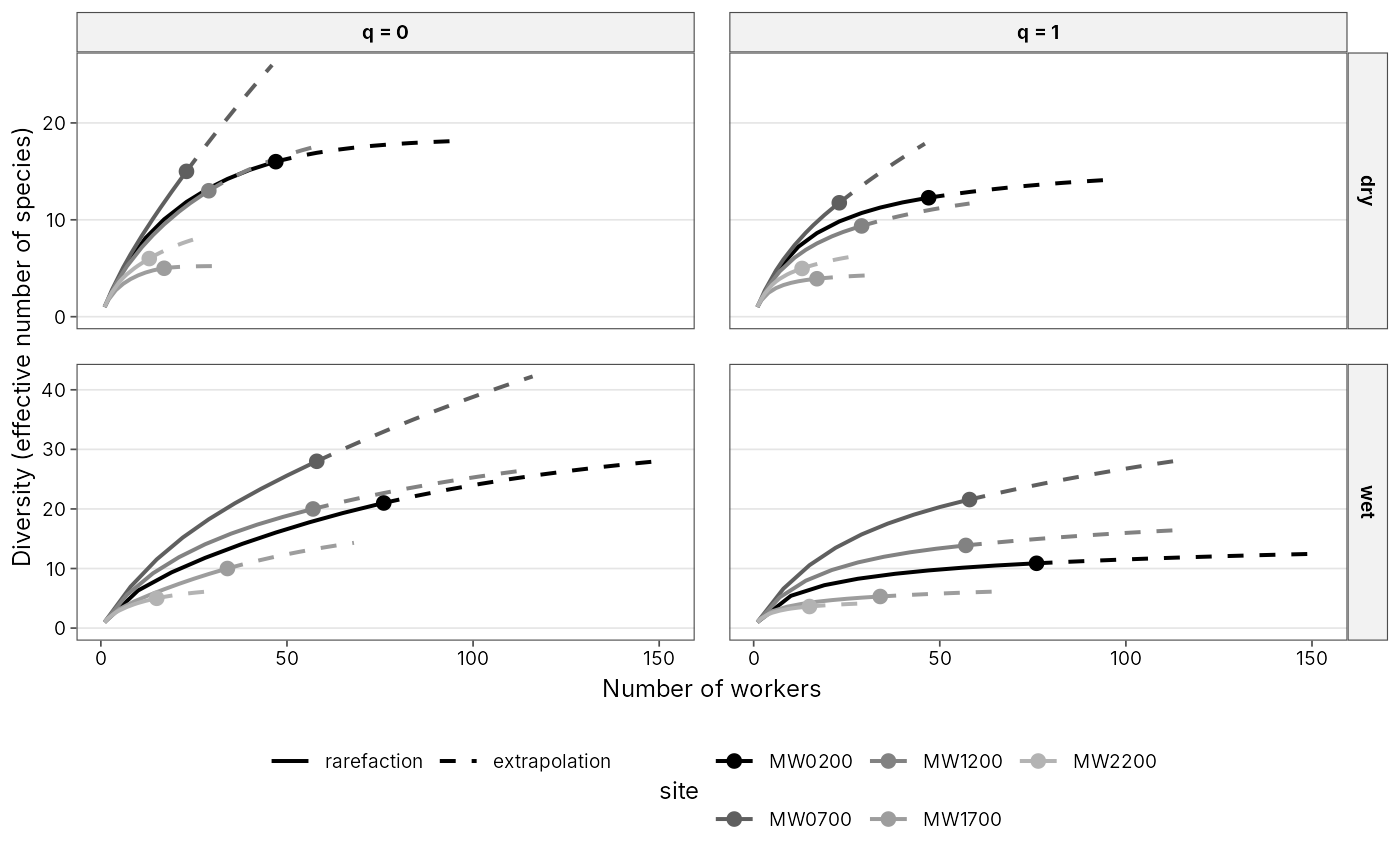
palette: Colours for sites or groups: "okabe_ito" (default), "grey", a character vector of colours, or NULL to keep the ggplot2 default so you can add your own scale.
theme: A ggplot2 theme added to the plot, by default theme_tidydiversity(). Use NULL to keep the ggplot2 default.
ci: Draw confidence intervals when the result has them.
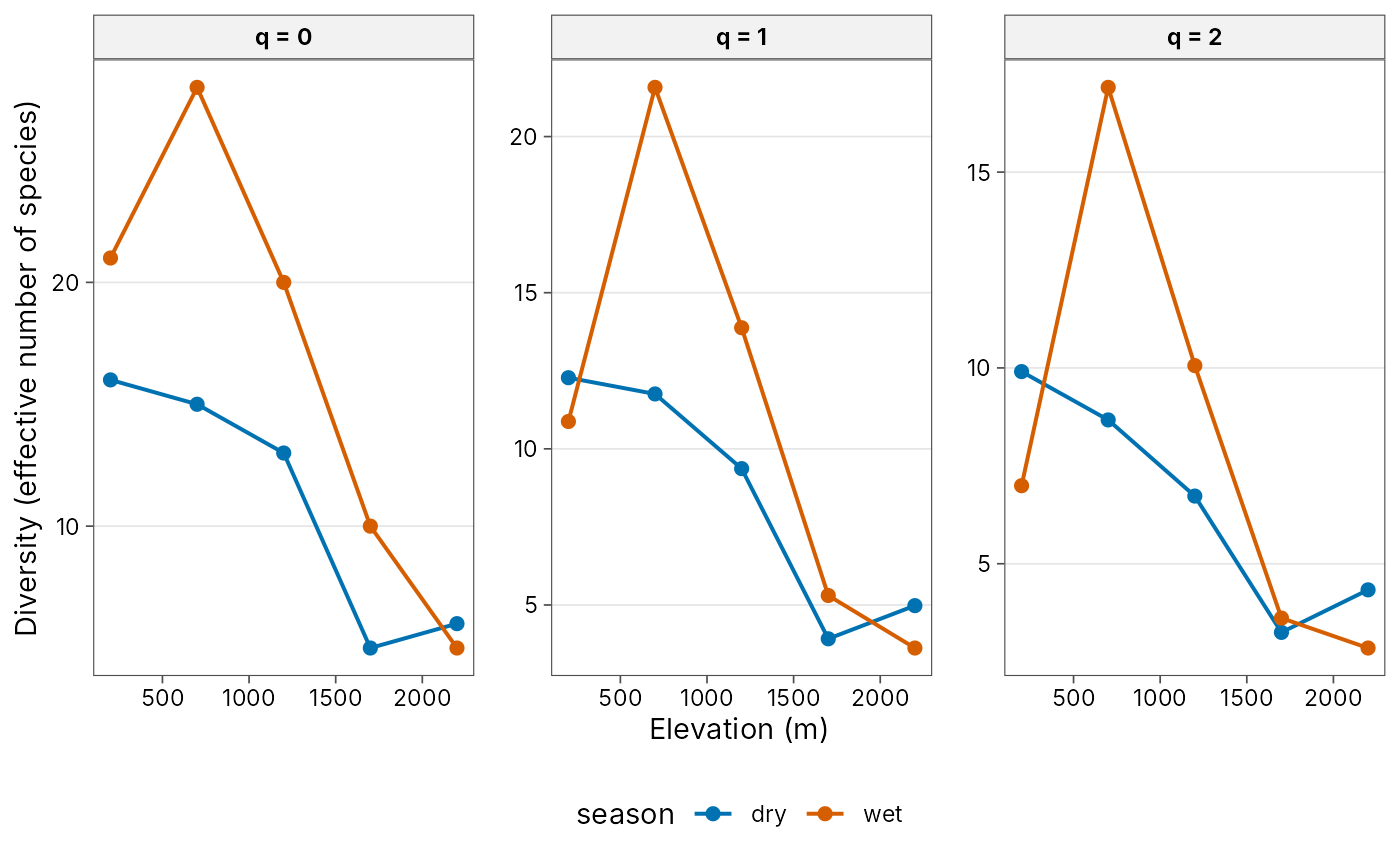
facet: For results with several orders q, facet by q (TRUE, the default) or draw all orders on one panel with q mapped to line type or shape (FALSE). Curves computed with .by groups are also faceted by group.
scales: Facet scales, passed to ggplot2::facet_wrap().
ncol: Number of facet columns.
xlab, ylab: Axis titles. The defaults describe the quantity and, where relevant, its unit.
...: Not used.
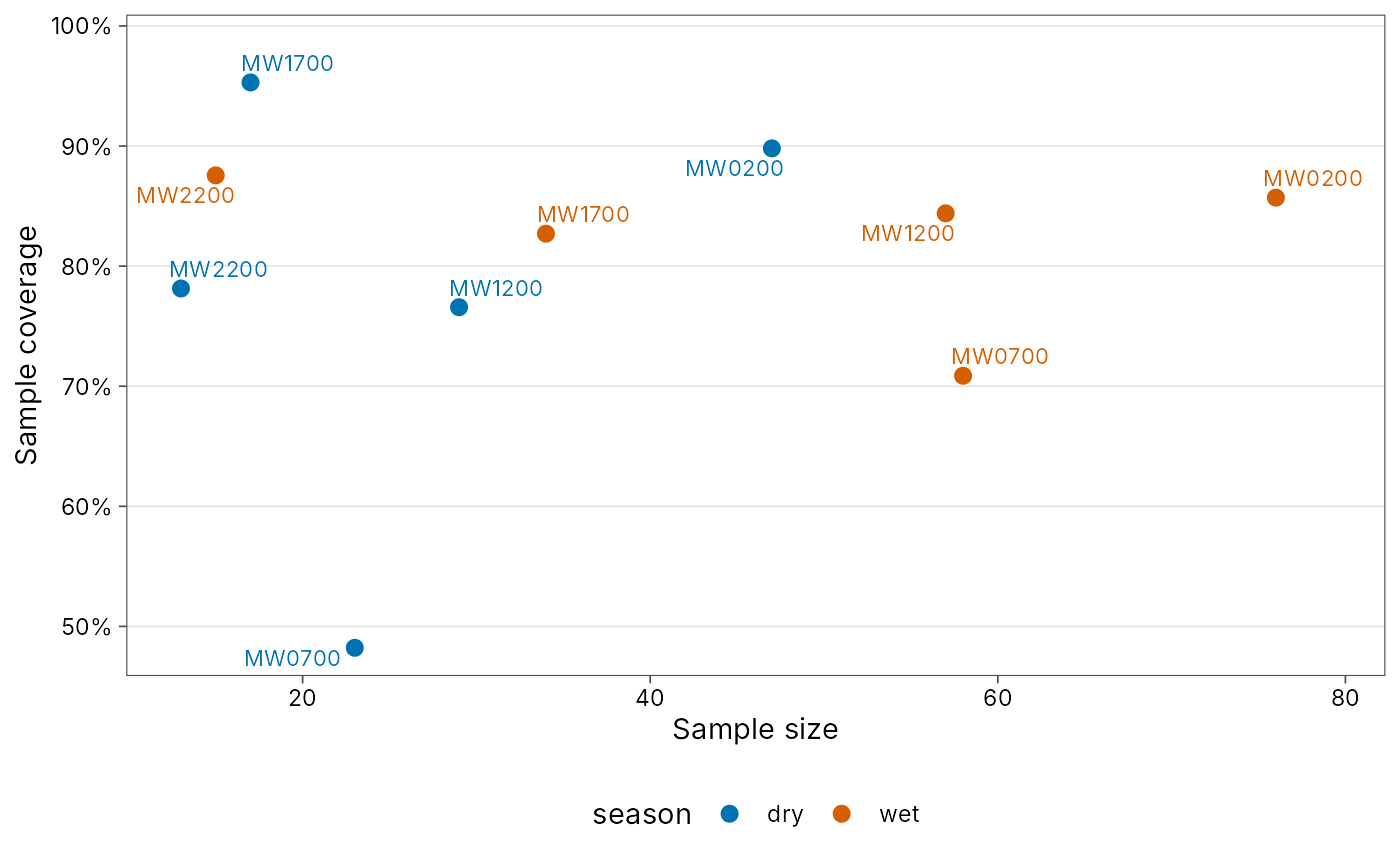
gradient: For div_hill() results, an optional numeric column (such as elevation, kept by .by) to plot diversity along.
labels: For div_coverage() results, label each point with its site; for beta_multi() results, print the turnover, nestedness and total values on the bars. Set to FALSE to leave them out.
component: For beta_pair() results, the component to map to colour: "total", "turnover" or "nestedness".
digits: For beta_multi() results, decimal places of the value labels.
what: For beta_hill() results, "diversity" (gamma, alpha and beta) or "dissimilarity" (the four normalised dissimilarities).

Value

A ggplot object.

Details

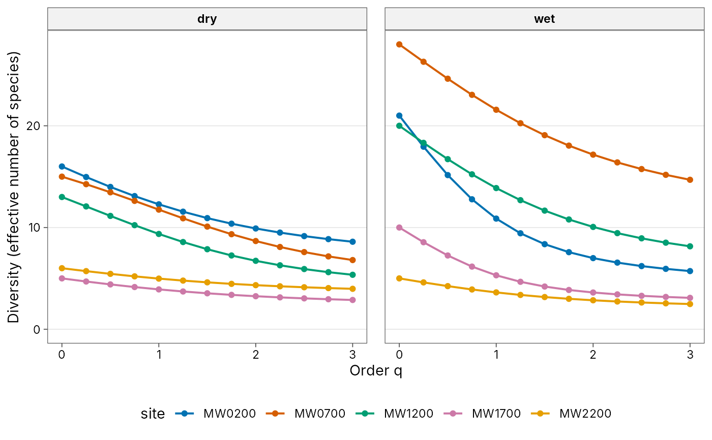
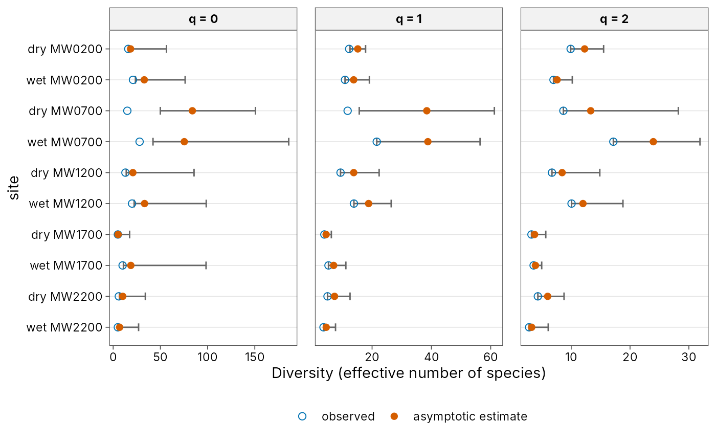
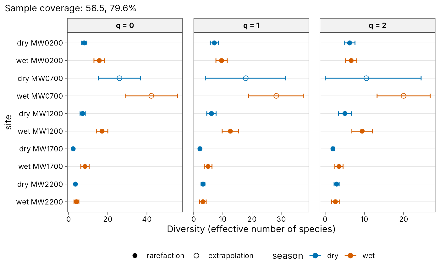
div_hill(): a Hill diversity profile across q, or diversity along a gradient column when gradient is given.
div_estimate(): observed and asymptotic diversity with intervals.
div_coverage(): sample coverage against sample size, points labelled by site.
div_rarefy(): rarefaction and extrapolation curves by sample size or by sample coverage.
div_standardise(): standardised diversity with intervals.
beta_pair(): a pairwise dissimilarity heatmap.
beta_multi(): multi-site turnover and nestedness as stacked bars, labelled with each component and the total.
beta_decay(): distance decay of dissimilarity components, with quasibinomial (logit-link) trends that stay within 0 to 1.
beta_hill(): gamma, alpha and beta diversity (or, with what = "dissimilarity", the four normalised dissimilarities) against the order q for each region, with bootstrap intervals when computed.

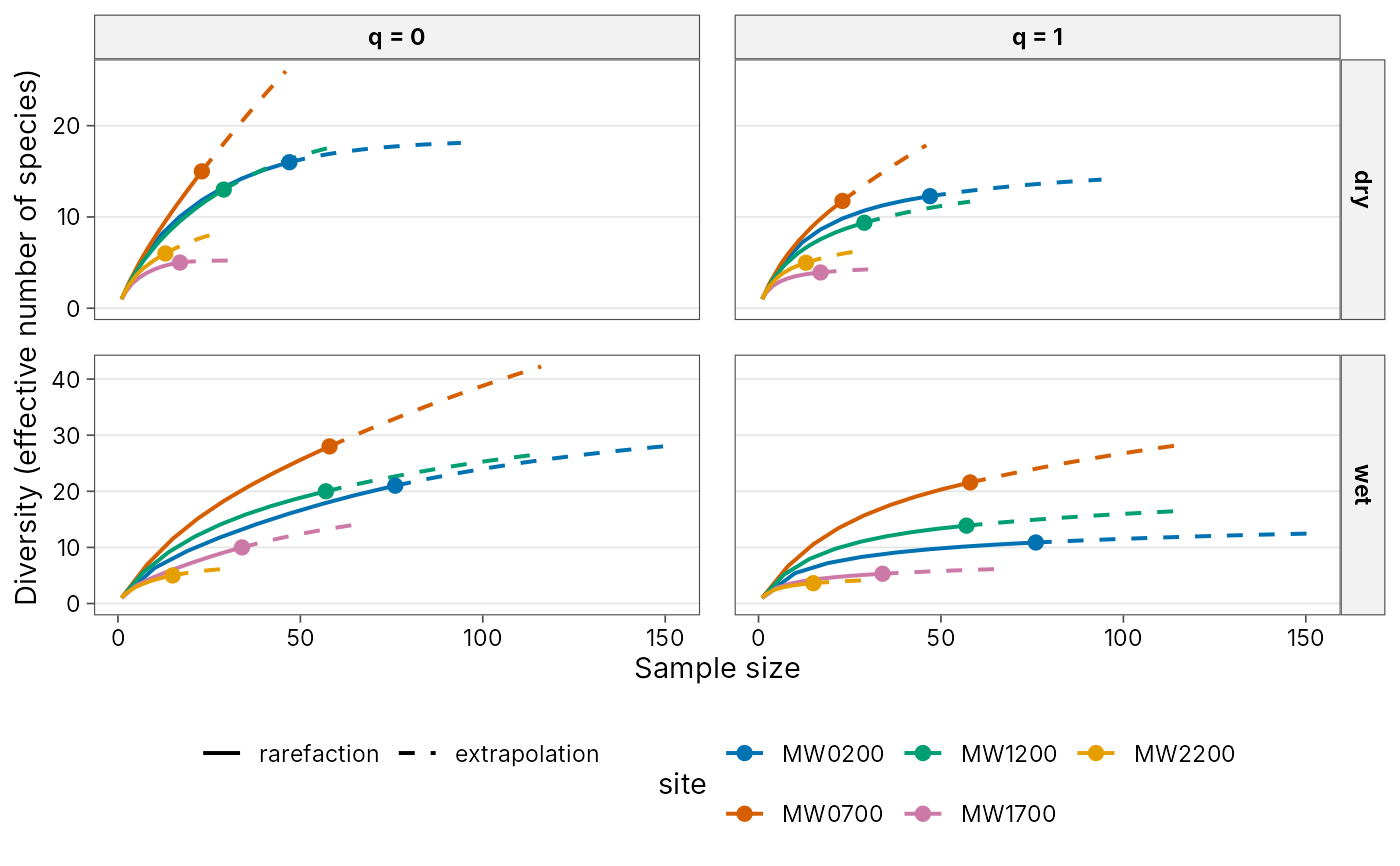
Every method returns an ordinary ggplot object, so labels, scales, themes and facets can be changed afterwards with +, for example + labs(x = "Number of workers"), and saved with ggplot2::ggsave(). The defaults use theme_tidydiversity() and the colour-blind-safe Okabe-Ito palette. Solid lines show rarefaction (interpolation), dashed lines extrapolation, points the observed sample, and shaded ribbons or bars the bootstrap confidence intervals when they were computed.

They need the ggplot2 package.

Examples

library(ggplot2)
curves <- div_rarefy(png_ants, q = c(0, 1), .by = season, knots = 20)
autoplot(curves)

autoplot(curves, x = "coverage")


# Customise like any ggplot
autoplot(curves, palette = "grey", ncol = 1) +
  labs(x = "Number of workers") +
  theme_tidydiversity(base_size = 9)


# \donttest{
div_hill(png_ants, q = seq(0, 3, by = 0.25), .by = season) |>
  autoplot()

div_hill(png_ants, .by = c(season, elevation)) |>
  autoplot(gradient = elevation, xlab = "Elevation (m)")


set.seed(1)
autoplot(div_estimate(png_ants, .by = season, nboot = 20))

autoplot(div_coverage(png_ants, .by = season))

autoplot(div_standardise(png_ants, .by = season, nboot = 20))


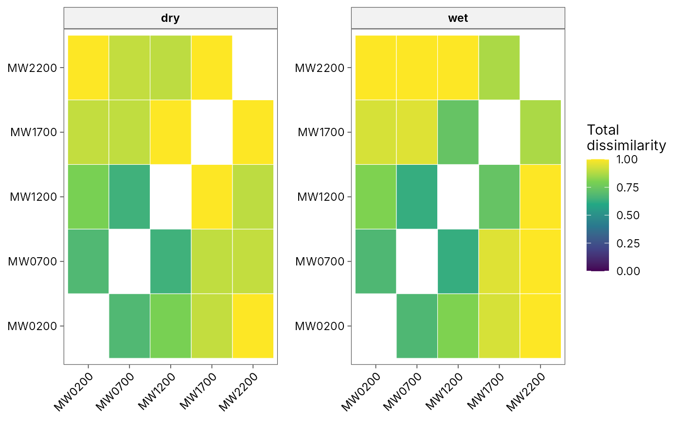
autoplot(beta_pair(png_ants, .by = season))

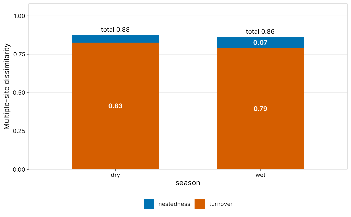
autoplot(beta_multi(png_ants, .by = season))


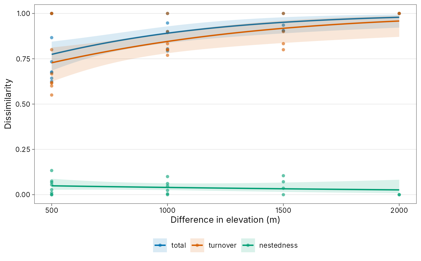
beta_decay(png_ants, gradient = elevation, .by = season) |>
  autoplot(xlab = "Difference in elevation (m)")

# }